In the previous lecture, we saw an algorithm to decide if one polygon is contractible, or if two polygons are homotopic, in the plane with several points removed. The algorithm runs in \(O(k\log k + nk)\) time, where \(k\) is the number of obstacle points; in the worst case, this running time is quadratic in the input size.
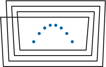
A running time of \(\Omega(nk)\) is inevitable if we are required to compute an explicit reduced crossing sequence; consider the polygon and obstacles below. But if a polygon is contractible—homotopic to a single point—its reduced crossing sequence is empty. Similarly the (non-reduced) crossing sequence of a polygon can have length \(\Omega(nk)\), even if the polygon is contractible, but nothing requires us to compute explicit crossing sequences!
In this lecture, I’ll describe another algorithm to test contractibility of polygons in punctured planes, which is faster either when the polygon has few self-intersections or when the number of obstacles is significantly larger than the number of polygon vertices. This algorithm is based on an algorithm of Cabello et al. [1], with some improvements by Efrat et al. [2]. Variations of this algorithm compute reduced crossing sequences without explicitly computing non-reduced crossing sequences first.
The key observation is that we are free to modify both the polygon and the obstacles, as long as our modifications do not change the reduced crossing sequence. In short, we are solving a topology problem, so we should feel free to choose whatever geometry is most convenient for our purposes.
To make the following discussion concrete, let \(O\) be an arbitrary set \(k\) of obstacle points in the plane, and let \(P\) be an arbitrary \(n\)-vertex polygon in \(\mathbb{R}^2 \setminus O\). As usual, we assume these objects are in general position: no two interesting points (obstacles, polygon vertices, or self-intersection points) lie on a common vertical line, and no three polygon vertices lie on a common line. In particular, no edge of \(P\) is vertical, and every point where \(P\) self-intersects is a transverse intersection between two edges. This assumption can be enforced with probability \(1\) by randomly rotating the coordinate system and randomly perturbing the vertices.
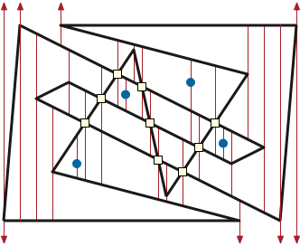
This first stage of our algorithm, like our earlier polygon triangulation algorithm, first constructs a trapezoidal decomposition of the input. We define the decomposition by extending vertical segments, which we call fences, upward and downward from each obstacle, from each vertex of \(P\), and from each self-intersection point of \(P\), until they hit edges of \(P\) (or escape to infinity). These fences, together with the edges of \(P\), decompose the plane into trapezoids, some of which are unbounded and others degenerate. See Figure 2.
A classical sweepline algorithm of Bentley and Ottmann constructs this decomposition in \(O((n + k + s)\log (n+k))\) time, where \(s\) is the number of self-intersection points. (There are several faster algorithms, especially when the number of self-intersections is small, but the Bentley-Ottmann algorithm is much simpler to describe and implement, and using these faster alternatives would not significantly improve the overall running time of our contractibility algorithm.)
Think of the \(n\) polygon edges and \(k\) obstacle points as \(n+k\) line segments (\(k\) of which have length zero). Any vertical line intersects t most \(n+1\) of these segments. The Bentley-Ottman algorithm sweeps a vertical line \(\ell\) across the plane, maintaining the sorted sequence of segments intersecting \(\ell\) in a balanced binary search tree, so that segments can be inserted or deleted in \(O(\log n)\) time. The \(x\)-coordinates where this intersection sequence changes are called events; there are two types of events:
The algorithm processes these events in order from left to right.
The vertices and obstacles are all known in advance, so after an initial \(O((n+k)\log(n+k))\) sorting phase, it is easy to find the next vertex event. Intersections are not known in advance, and computing them by brute force in \(O(n^2)\) time would take too long. Instead, we observe that the next intersection event must occur at the intersection of two consecutive segments along \(\ell\). Thus, for each consecutive pair of segments that intersects to the right of \(\ell\), we have a potential intersection event. We maintain these \(O(n)\) potential intersection events in a priority queue, so that we can find the next actual intersection event in \(O(\log n)\) time.
At each event, we insert a single fence, perform \(O(1)\) binary-tree operations to maintain the intersection sequence with \(\ell\), and then perform \(O(1)\) priority-queue operations. There are \(O(n + k + s)\) events, each requiring \(O(\log n)\) time, so including the initial sort, the overall running time is \(O((n + k + s)\log (n + k))\).
As a by-product of the sweep-line algorithm, we obtain the complete list of self-intersection points. We subdivide \(P\) by introducing two coincident vertices at each self-intersection point, increasing the number of vertices from \(n\) to \(n+2s\), and ensuring that the edges of \(P\) intersect only at vertices.
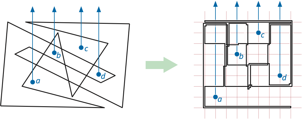
Next, we replace \(P\) and \(O\) with a new orthogonal polygon \(\bar{P}\) and a new set of obstacles \(\bar{O}\) that define exactly the same crossing sequence. At a high level, we replace each edge of \(P\) with a horizontal line segment and each vertex of \(P\) with a vertical line segment.
The \(y\)-coordinates of the horizontal segments are determined by the following vertical ranking of the polygon edges and obstacle points. Let \(S\) be the set of \(m = n+2s+k\) interior-disjoint segments, consisting of the subdivided edges of \(P\) and the obstacles \(O\). For any two segments \(\sigma\) and \(\tau\) in \(S\), write \(\sigma\Uparrow\tau\) (and say “sigma is above tau”) if there is a vertical segment with positive length whose upper endpoint lies on \(\sigma\) and whose lower endpoint lies on \(\tau\).
Rotate the indices if necessary, so that the right endpoint of \(\sigma_1\) has strictly smaller \(x\)-coordinate than the right endpoint of any other segment \(\sigma_i\) in the cycle. In particular, the right endpoints of \(\sigma_2\) and \(\sigma_r\) are both strictly to the right of \(\sigma_1\). Thus, the right endpoint of \(\sigma_1\) is both directly above some point of \(\sigma_2\) and directly below some point of \(\sigma_r\). It follows that \(\sigma_r \Uparrow \sigma_2\), which contradicts the minimality of the cycle.
Now write \(\sigma\uparrow \tau\) (and say “sigma is immediately above tau”) of some fence in the trapezoidal decomposition of \(S\) touches both \(\sigma\) and \(\tau\), and in particular touches \(\sigma\) above the point where it touches \(\tau\). Because \(\sigma\uparrow \tau\) immediately implies \(\sigma\Uparrow \tau\), the relation \(\uparrow\) is also acyclic; in fact, our earlier relation \(\Uparrow\) is the transitive closure of \(\uparrow\). We can easily extract a directed acyclic graph \(G^\uparrow\) representing the relation \(\uparrow\) (and thus its transitive closure \(\Uparrow\)) directly from the trapezoidal decomposition of \(S\).
(Any linear extension of \(\Uparrow\) is called a of \(D\); the previous lemma implies that such an order always exists.)
Now index the segments \(S = \{\sigma_1, \sigma_2, \dots, \sigma_m \}\) according to an arbitrary topological ordering of the graph \(G^\uparrow\), so that \(\sigma_i \Uparrow \sigma_j\) implies \(i < j\). For any segment \(\sigma_i\), let \(\textsf{obsbelow}(\sigma_i)\) denote the number of obstacle segments \(\sigma_j\) such that \(j < i\). Finally, we define the vertical rank \(\textsf{vrank}(\sigma_i)\) as follows:
Thus, all vertical ranks are integers between \(0\) and \(2k\), every obstacle has odd vertical rank, and every polygon edge has even vertical rank.
We also define the horizontal rank of any polygon vertex or an obstacle point \(p\) as follows. Let \(\textsf{obsleft}(p)\) to be the number of obstacles with strictly smaller \(x\)-coordinates than \(p\).
Thus, all horizontal ranks are integers between \(0\) and \(2k\), every obstacle has odd horizontal rank, and every polygon vertex has even horizontal rank.
Now we define a rectified polygon \(\bar{P}\) and new obstacles \(\bar{O}\) as follows:
Replace each edge \(pq\) of \(P\) with a horizontal segment between \((\textsf{hrank}(p), \textsf{vrank}(pq))\) and \((\textsf{hrank}(q), \textsf{vrank}(pq))\). Similarly, replace each vertex \(q\) of \(P\), with adjacent edges \(pq\) and \(qr\), with a vertical segment between \((\textsf{hrank}(q), \textsf{vrank}(pq))\) and \((\textsf{hrank}(q), \textsf{vrank}(qr))\). Connecting these horizontal and vertical segments in sequence around \(P\) gives us an orthogonal polygon \(\bar{P}\).
For each obstacle \(o\), let \(\bar{o} = (\textsf{hrank}(o), \textsf{vrank}(o))\). The set of all such points is our new obstacle set \(\bar{O}\).
By construction, every vertex of \(\bar{P}\) has even integer coordinates, and every obstacle in \(\bar{O}\) has odd integer coordinates, so \(\bar{P}\) is a polygon in \(\mathbb{R}^2\setminus \bar{O}\). Moreover, the crossing sequence of the rectified polygon \(\bar{P}\) with respect to the new obstacles \(\bar{O}\) is identical to the crossing sequence of the original polygon \(P\) with respect to the original obstacles \(O\). Thus, \(P\) is contractible in \(\mathbb{R}^2\setminus O\) if and only if \(\bar{P}\) is contractible in \(\mathbb{R}^2\setminus \bar{O}\).
It is actually possible to construct an explicit deformation of \(P\) and \(O\) into \(\bar{P}\) and \(\bar{O}\), as a sequence of elementary moves of two types: safe vertex moves (translate a vertex of \(P\) without touching any obstacle) and “safe obstacle moves” (translate one obstacle in \(O\) without touching \(P\)). Moreover, we can guarantee that throughout the entire deformation, the crossing sequence of the polygon with respect to the obstacles remains unchanged. Fortunately, we don’t actually need an explicit homotopy; the invariance of the crossing sequence is enough.
So why did we go through this madness? We have now reduced our problem from arbitrary polygons to particularly well-behaved orthogonal polygons. Restricting to orthogonal polygons allows us to represent and manipulate the crossing sequence of \(\bar{P}\) implicitly using relatively simple data structures.
Let \(\bar{n} = 2n+4s\) denote the number of vertices in the rectified polygon \(\bar{P}\). Without loss of generality, we can assume that the \(i\)th edge \(\bar{p}_i \bar{p}_{i+1}\) of \(\bar{P}\) is horizontal if \(i\) is even and vertical if \(i\) is odd. Thus, we can represent \(\bar{P}\) itself using an alternating sequence of \(x\)- and \(y\)-coordinates: \[ x_0, y_1, x_2, y_3, \dots, x_{\bar{n}-2}, y_{\bar{n}-1}, \] where \(\bar{p}_i = (x_i, y_{i+1})\) if \(i\) is even, and \(\bar{p}_i = (x_{i+1}, y_i)\) if \(i\) is odd. We store these coordinates in any data structure that allows us to change one coordinate or remove any adjacent pair of coordinates \(x_i, y_{i\pm 1}\) in \(O(1)\) time—for example, a circular doubly-linked list.
We now reduce \(\bar{P}\) by repeatedly applying two operations, called eliding and sliding, which simplify the polygon without changing its homotopy class. Each operation requires \(O(\log k)\) time, and the reduction requires at most \(O(\bar{n})\) of these operations, so the overall reduction time is is \(O(\bar{n}\log k) = O((n+s)\log k)\). If the reduced polygon is empty, we correctly report that \(P\) is contractible; otherwise, we correctly report that \(P\) is not contractible.
This makes the pictures nicer, but it isn’t actually necessary; consider removing.
The rectified polygon \(\bar{P}\) can contain edges with length zero; we elide (that is, remove) all such edges in a preprocessing phase. Geometrically, there are two types of zero-length edges:
However, our representation of \(\bar{P}\) as a list of alternating \(x\)- and \(y\)-coordinates allows us to treat these two cases identically in \(O(1)\) time. To remove the zero-length edge edge \(\bar{p}_{i-1}\bar{p}_i\), we delete the \((i-1)\)th and \(i\)th coordinates from our coordinate list. Specifically:
Equivalently, we can remove any zero-length edge \(\bar{p}_{i-1}\bar{p}_i\) using two safe vertex moves:
We can remove all zero-length edges from \(\bar{P}\) in \(O(\bar{n})\) time using a “left-greedy” algorithm similar to the crossing-word reduction algorithm in the previous lecture.
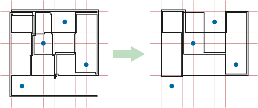
We call a positive-length edge of \(\bar{P}\) a bracket if both of its neighboring edges are on the same side of the line through the edge. That is, the edge and its neighbors look like \(\sqcup\), \(\sqsubset\), \(\sqcap\), or \(\sqsupset\). Sliding a bracket moves it as far inward as possible, shortening the neighboring edges, until at least one of two conditions is met:
The bracket has distance \(1\) from an obstacle inside the bracket; we call such a bracket frozen. Sliding a frozen bracket further would change the crossing sequence of \(\bar{P}\) by either adding or deleting a single crossing, thereby changing the homotopy class.
At least one of the edges adjacent to the bracket has length zero, which we can safely elide, just as in the previous phase. (If the zero-length edge is a spur, several elisions may be required to ensure that all edges have positive length.)
Sliding a bracket requires changing exactly one coordinate in our alternating coordinate list, and then deleting zero or more pairs of coordinates (to elide zero-length edges created by the slide).
The reduction algorithm ends either when all remaining brackets are frozen (and all edges have positive length), or when no edges are left at all. For example, if \(\bar{P}\) is a rectangle that doesn’t not contain any obstacles, the first bracket slide creates two zero-length edges; eliding these edges removes every edge from the polygon.
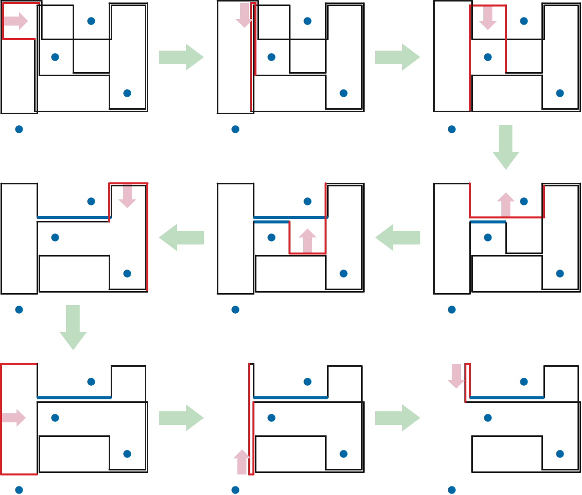
Because each bracket slide (and ensuing elisions) either freezes a bracket or decreases the number of polygon vertices, the reduction ends after at most after \(O(\bar{n})\) bracket slides. (A bracket slide can increase the number of polygon self-intersections, but we don’t care about that; we only needed to find self-intersections so that we could compute vertical ranks.) The figure on the next page shows a sequence of bracket slides contracting a rectified cycle.
The correctness of this algorithm rests on the following lemma.
The other direction is more interesting. We actually need to reason about the crossing sequence defined by both upward and downward rays from each obstacle. Suppose \(\bar{P}\) is contractible. Then our earlier arguments imply that the mixed crossing sequence of \(\bar{P}\) can be reduced to the empty string, suing exactly the same algorithm as usual. There are two cases to consider.
First suppose both mixed crossing sequences of \(\bar{P}\) is actually empty. Then \(\bar{P}\) does not cross the vertical line through any obstacle. It follows that every vertex of \(\bar{P}\) has the same even \(x\)-coordinate, and thus every “horizontal” edge of \(\bar{P}\) has length zero. It follows by induction that \(\bar{P}\) can be reduced to a single point by eliding every horizontal edge.
Otherwise, because \(\bar{P}\) is contractible, its mixed crossing sequence contains an elementary reduction. So there must be a subpath of \(\bar{P}\) that crosses the same obstacle ray twice in a row, without crossing the vertical line through any obstacle in between. (These two crossings would be canceled by an elementary reduction.) Without loss of generality, suppose this subpath crosses some upward obstacle ray from right to left, and then crosses that same ray from left to tight. Then the leftmost vertical edge of that subpath forms a bracket, and sliding that bracket reduces the complexity of either the polygon or its crossing sequence. It follows by induction that \(\bar{P}\) can be reduced to a polygon with an empty crossing sequence, and thus to a single point.
A close reading of this proof reveals that we only ever need to perform horizontal bracket slides; even eliding zero-length edges is unnecessary.
To implement bracket slides efficiently, we preprocess the rectified obstacles \(\bar{O}\) that supports fast queries of the following form: Given a horizontal query segment \(\sigma\), report the lowest obstacle (if any) that lies directly above \(\sigma\). Symmetric data structures can report the highest sentinel point below a horizontal segment, or the closest sentinel points to the left and right of a vertical segment.
Lemma: Any set \(\bar{O}\) of \(k\) points in the plane can be preprocessed in \(O(k\log k)\) time into a data structure of size \(O(k\log k)\), so that the lowest point (if any) above an arbitrary horizontal query segment can be computed in \(O(\log k)\) time.
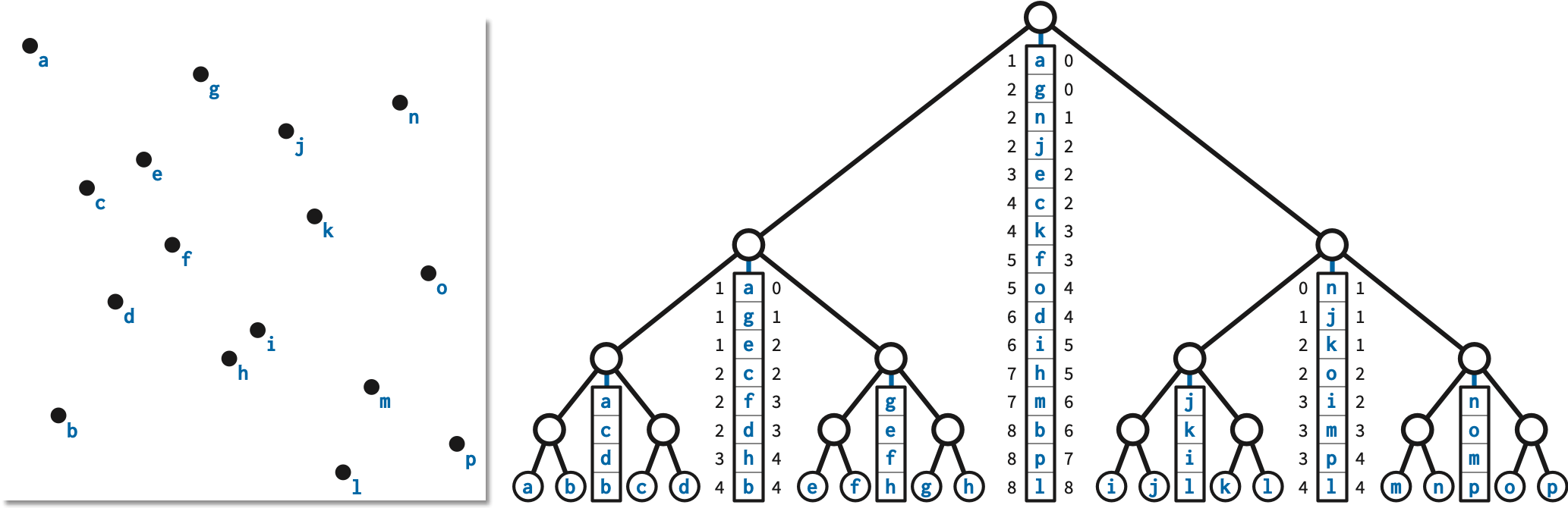
For each node \(v\) of \(T\), let \(l_v\) and \(r_v\) denote the smallest and largest \(x\)-coordinates in stored in the subtree rooted at \(v\), and let \(\bar{O}_v\) denote the subset of obstacle points with \(x\)-coordinates between \(l_v\) and \(r_v\). Each node \(v\) in \(T\) stores the following information, in addition to the search key \(x_v\).
It is possible to construct a layered range tree for \(\bar{O}\) in \(O(k\log k)\) time; the total size of the data structure is also \(O(k\log k)\).
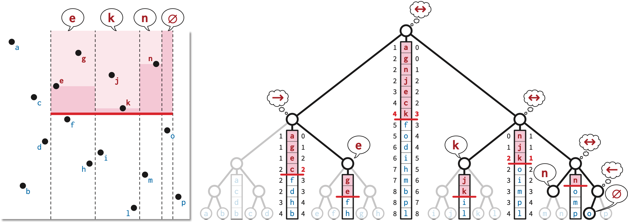
Now consider a query segment \(\sigma\) with endpoints \((l,b)\) and \((r,b)\) with \(l<r\). We call a node \(v\) active for this segment if \(l_v\le l\) and \(r\le r_v\), but the parent of \(v\) is not active. There are at most two active nodes at each level of the tree, so there are \(O(\log k)\) active nodes altogether. We can easily find these active nodes in \(O(\log h)\) time by searching down from the root.
For any node \(v\), let \(\textsf{lowest}(v,b)\) denote the index of the lowest point in \(\bar{O}_v\) that lies above the line \(y=b\), or \(0\) if there is no such point. We can compute \(\textsf{lowest}(\textsf{root}(T),b)\) in \(O(\log h)\) time by binary search; for any other node \(v\), we can compute \(\textsf{lowest}(v,b)\) in \(O(1)\) time from \(\textsf{lowest}(\textsf{parent}(v), b)\) and the left or right ranks stored at \(\textsf{parent}(v)\). Thus, we can compute \(\textsf{lowest}(v,b)\) for every active node \(v\) in \(O(\log h)\) time. The answer to our query is the lowest of these \(O(\log h)\) points.
Now let’s put all the ingredients of the algorithm together. Recall that the original input is a set \(O\) containing \(k\) sentinel points, and a polygon \(P\) in \(\mathbb{R}^2\setminus O\).
First we sort the obstacles in \(O\) from left to right in \(O(k\log k)\) time.
Next we compute the trapezoidal decomposition of \(P\) and \(O\) using the Bentley-Ottmann sweepline algorithm in \(O((n+k+s)\log (n+k))\) time, where \(s\) is the number of self-intersection points of \(P\). We subdivide the edges of \(P\) at its self-intersection points, increasing the number of vertices of \(P\) to \(m = n + 2s\).
Then we compute the vertical ranks of the obstacles and the edges of \(P\) in \(O(m+k) = O(n+k+s)\) time. We also compute the horizontal ranks of the obstacles and the vertices of \(P\) in \(O(m \log m + k)\) time, by sorting the vertices of \(P\) and merging them with the sorted list of obstacles.
Next we compute the rectified polygon \(\bar{P}\) and obstacles \(\bar{O}\) in \(O(m + k)\) time.
Then, we reduce \(\bar{P}\) as much as possible by eliding zero-length edges and sliding brackets. After an \(O(m)\)-time initial pass, each elision takes \(O(1)\) time, and each bracket slide takes \(O(\log k)\) time. Each operation either freezes a bracket or reduces the complexity of \(\bar{P}\), so after \(O(m)\) operations, performed in \(O(m\log k)\) time, \(\bar{P}\) is reduced as much as possible.
Finally, we report that \(P\) is contractible if and only if the reduced rectified polygon is empty.
Altogether, this algorithm runs in \(O((n+k+s)\log(n+k))\) time.
This is faster than the brute-force reduction algorithm from the previous lecture when either the polygon has few self-intersections or the number of obstacles is significantly larger than the number of polygon vertices. Specifically, the running time of the new algorithm is smaller than the old running time \(O(k\log k + nk)\) whenever \(s = o(nk/\log(n+k))\). Even in the worst case, when \(s = \Theta(n^2)\), the running time of the new algorithm simplifies to \(O((k+n^2)\log(n+k))\), which is still smaller than \(O(k\log k + nk)\) when \(n = o(k/log n)\).
Extracting reduced crossing sequences from the reduced rectified polygon.
Testing if a polygon made from two (almost) simple paths is contractible.
Testing if two polygons, each with few self-intersections, are homotopic.
Faster three-sided range query structures for integer points and ranges.
Avoiding computing self-intersections (Bespanyatnikh)
Sergio Cabello, Yuanxin Liu, Andrea Mantler, and Jack Snoeyink. Testing homotopy for paths in the plane. Discrete Comput. Geom. 31(1):61–81, 2004.
Alon Efrat, Stephen G. Kobourov, and Anna Lubiw. Computing homotopic shortest paths efficiently. Comput. Geom. Theory Appl. 35(3):162–172, 2006. arXiv:cs/0204050.
Dan E. Willard. New data structures for orthogonal range queries. SIAM J. Comput. 24 14(1):232–253, 1985. Layered range trees.