A graph is an abstract combinatorial structure that models pairwise relationships. You probably have a good intuitive idea what a graph is already. Nevertheless, to avoid subtle but pervasive differences in terminology, notation, and basic assumptions, I will carefully define everything from scratch. In particular, we need a definition that allows parallel edges and loops, so we can’t use the standard combinatorialist’s definition as a pair of sets \((V,E)\), and I don’t want to wander into the notational quagmire of multisets. So here we go.
An abstract graph is a quadruple \(G := (V, D, \textsf{rev}, \textsf{head})\), where
Darts are also called half-edges or arcs or brins (French for “strands”).
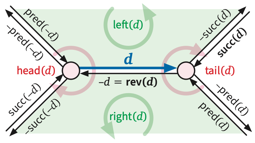
For any dart \(d\), we call the dart \(\textsf{rev}(d)\) the reversal of \(d\), and we call the vertex \(\textsf{head}(d)\) the head of \(d\). The tail of a dart is the head of its reversal: \(\textsf{tail}(d) := \textsf{head}(\textsf{rev}(d))\). The head and tail of a dart are its endpoints. Intuitively, a dart is a directed path from its tail to its head; in keeping with this intuition, we say that a dart \(d\) leaves its tail and enters its head. I often write \(u\mathord\to v\) to denote a dart with tail \(u\) and head \(v\), even (at the risk of confusing the reader) when there is more than one such dart.
For any dart \(d\in D\), the unordered pair \(|d| = \{d,\textsf{rev}(d)\}\) is called an edge of the graph. We often write \(E\) to denote the set of edges of a graph. The constituent darts of an edge \(e\) are arbitrarily denoted \(e^+\) and \(e^-\). The endpoints of an edge \(e = \{ e^+, e^- \}\) are the endpoints (equivalently, just the heads) of its constituent darts. Intuitively, each dart is an orientation of some edge from one of its endpoints to the other.
A vertex \(v\) and an edge \(e\) are incident if \(v\) is an endpoint of \(e\); two vertices are neighbors if they are endpoints of the same edge. We often write \(uv\) to denote an edge with endpoints \(u\) and \(v\), even (at the risk of confusing the reader) when there is more than one such edge.
A loop is an edge \(e\) with only one endpoint, that is, \(\textsf{head}(e^+) = \textsf{tail}(e^+)\). Two edges are parallel if they have the same endpoints. A graph is simple if it has no loops or parallel edges, and non-simple otherwise. Non-simple graphs are sometimes called “generalized graphs” or “multigraphs”; I will just call them “graphs”.
Let me repeat this louder for the kids in the back: Graphs are not necessarily simple.
The degree of a vertex \(v\), denoted \(\deg_G(v)\) (or just \(\deg(v)\) if the graph \(G\) is clear from context), is the number1 of darts whose head is \(v\), or equivalently, the number of incident edges plus the number of incident loops. A vertex is isolated if it is not incident to any edge.
Here is an equivalent definition that might be clearer to computer scientists: A (finite) graph is whatever can be stored in a standard graph data structure.
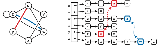
The canonical textbook graph data structure is the incidence list. (For simple graphs, the same data structure is more commonly called an adjacency list.) The \(n\) vertices of the graph are represented by distinct integers between \(1\) and \(n\). A standard incidence list consists of an array indexed by the vertices; each array entry in the array points to a linked list of the darts leaving the corresponding vertex. (The order of darts in these linked lists is unimportant; we use linked lists only because they support certain operations quickly.) The record for each dart \(d\) contains the index of \(\textsf{head}(d)\) and a pointer to the record for \(\textsf{rev}(d)\). Storing a graph with \(n\) vertices and \(m\) edges in an incidence list requires \(O(n + m)\) space.
If a graph is stored in an incidence list, we can insert a new edge in \(O(1)\) time, delete an edge in \(O(1)\) time (given a pointer to one of its darts), and visit all the edges incident to any vertex \(v\) in \(O(1)\) time per edge, or \(O(\deg(v))\) time altogether. There are a few standard operations that incidence lists do not support on \(O(1)\) time, the most glaring of which is testing whether two vertices are neighbors. Surprisingly, however, most efficient graph algorithms do not require this operation, and for those few that do, we can replace the linked lists with hash tables.
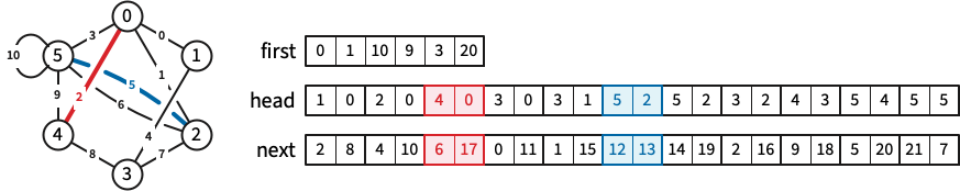
More generally, “array” and “linked list” can be replaced by any suitable data structures that allow random access and fast iteration, respectively. A particularly simple and efficient implementation keeps all data in standard arrays. For a graph with \(n\) vertices and \(m\) edges, we represent vertices by integers between \(0\) and \(n-1\), edges by integers from \(0\) to \(m-1\), and darts by integers between \(0\) and \(2m-1\). Each edge \(e\) is composed of darts \(e^- = 2e\) and \(e^+ = 2e+1\); thus, the reversal of any dart \(d\) is obtained by flipping its least significant bit: \(d\oplus 1\). The actual data structure consists of three arrays:
It is convenient to treat the list of darts leaving each vertex as a circular list; then \(\textsf{next}\) stores a permutation of the darts, each of whose cycles is the set of darts leaving a vertex. We may also want to store a predecessor array \(\textsf{prev}[0..2m-1]\) that stores the inverse of this permutation. We do not need a separate \(\textsf{tail}\) array, because \(\textsf{tail}(d) = \textsf{head}[d \oplus 1]\).
For algorithms that make frequent changes to the graph (adding and/or deleting vertices and/or edges), we should use dynamic hash tables instead of raw arrays. Finally, we can easily store algorithm-dependent auxiliary data such as vertex coordinates, edge weights, distances, or flow capacities in separate arrays (or hash tables) indexed by vertices, edges, or darts, as appropriate.
Graphs can also be formalized as topological structures rather than purely combinatorial structures. Informally, a topological graph consists of a set of distinct points called vertices, together with a collection of vertex-to-vertex paths called edges, which are disjoint and simple, except possibly at their endpoints.
More formally, a topological graph \(G^\top\) is the quotient space of a set of disjoint closed intervals, with respect to an equivalence relation over the intervals’ endpoints. The projections of the intervals are the edges of \(G^\top\); the projections (or equivalence classes) of interval endpoints are the vertices of \(G^\top\). Again, for the kids in the back, topological graphs are not required to be simple; they can contain loops and parallel edges.2
Mechanical definition-chasing implies that any topological graph \(G^\top\) can be described by a unique abstract graph \(G\), For example, the darts of \(G\) are orientations of the edges of \(G^\top\). Conversely, any abstract graph describes a unique (up to homeomorphism) topological graph \(G^\top\).3
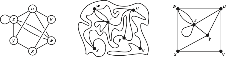
A planar embedding of a graph \(G\) represents its vertices as distinct points in the plane (typically drawn as small circles) and its edges as simple interior-disjoint paths between their endpoints. Equivalently, a planar embedding of \(G\) is a continuous injective function from the corresponding topological graph \(G^\top\) into the plane. A graph is planar it it has at least one planar embedding. Somewhat confusingly, the image of a planar embedding of a planar graph is also called a plane graph.
The components of the complement of the image of a planar embedding are called the faces of the embedding. Assuming the embedded graph is connected, the Jordan curve theorem implies that every bounded face is homeomorphic to an open disk, and the unique unbounded face is homeomorphic to the complement of a closed disk. For disconnected graphs, at least one face is homeomorphic to an open disk with a finite number of closed disks removed.
The faces on either side of an edge of a planar embedding are called the shores of that edge. For any dart \(d\), the face just to the left of the image of \(d\) in the embedding is the left shore of \(d\), denoted \(\textsf{left}(d)\); symmetrically, the face just to the right is the right shore \(\textsf{right}(d)\). The left and right shores of a dart can be the same face. An edge \(e\) and a face \(f\) are incident if \(f\) is one of the shores of \(e^+\); similarly, an vertex \(v\) and a face \(f\) are incident if \(v\) and \(f\) have a common incident edge. The degree of a face \(f\), denoted \(\deg_G(f)\) (or just \(\deg(f)\) if \(G\) is clear from context), is the number of darts whose right shore is \(f\).
Let \(F\) be the set of faces of a planar embedding of a connected graph with vertices \(V\) and edges \(E\). The decomposition of the plane into vertices, edges, and faces, typically written as a triple \((V,E,F)\), is called a planar map. Trapezoidal decompositions and triangulations of polygons are both examples of planar maps. A planar map is called a triangulation if every face, including the outer face, has degree \(3\). The underlying graph \((V, E)\) of a planar triangulation is not necessarily simple.4
As usual in topology, we are not really interested in particular embeddings or maps, but rather topological equivalence classes of embeddings or maps. Two planar embeddings of the same graph \(G\) are considered equivalent if there is an orientation-preserving homeomorphism of the plane to itself that carries one embedding to the other, or equivalently, if one embedding can be continuously deformed to the other through a continuous family of embeddings. Fortunately, every equivalence class of embeddings has a concrete combinatorial representation, called a rotation system.
Recall that a permutation of a finite set \(X\) is a bijection \(\pi\colon X \to X\). For any permutation \(\pi\) and any element \(x\in X\), let \(\pi^0(x) := x\) and \(\pi^k(x) := \pi(\pi^{k-1}(x))\) for any integer \(k > 0\). The orbit of an element \(x\) is the set \(\{\pi^k(x) \mid k\in\mathbb{N}\} = \{x, \pi(x), \pi^2(x), \dots\}\). The restriction of \(\pi\) to any of its orbits is a cyclic permutation; the infinite sequence \(x,\pi(x),\pi^2(x),\dots\) repeatedly cycles through the elements of the orbit of \(x\). Thus, the orbits of any two elements of \(X\) are either identical or disjoint.
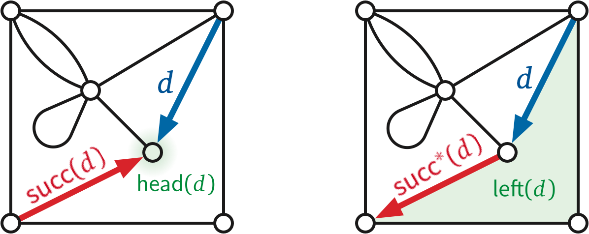
The successor permutation or an embedding of \(G\) is a permutation of the darts of \(G\); specifically, the successor \(\textsf{succ}(d)\) of any dart \(d\) is the successor of \(d\) in the clockwise sequence of darts entering \(\textsf{head}(d)\).5
Finally, the rotation system of an embedding is a triple \(\Sigma = (D, \textsf{rev}, \textsf{succ})\), where
More generally, a rotation system or combinatorial map is any triple \((D, \textsf{rev}, \textsf{succ})\) where \(D\) is a set, \(\textsf{rev}\) is a fixed-point-free involution of \(D\), and \(\textsf{succ}\) is another permutation of \(D\). The vertices of a combinatorial map are the orbits of \(\textsf{succ}\), its edges are the orbits of \(\textsf{rev}\), and its faces are the orbits of \(\textsf{rev}(\textsf{succ})\). The vertices and edges define the 1-skeleton or underlying graph of \(\Sigma\).
In other words, a rotation system is (almost) an incidence list where the order of darts in each list actually matters! The only annoying discrepancy is that rotation systems order darts into each vertex, while incidence lists order darts out of each vertex, but we can easily translate between these two standards using the identity \(\textsf{next}(d) = \textsf{rev}(\textsf{succ}(\textsf{rev}(d)))\).
The of any connected graph embedding are also implicitly encoded in its rotation system. Recall that \(\textsf{rev}\) is the reversal permutation of the darts of a graph. For any dart \(d\), the dual successor \(\textsf{succ}^*(d):= \textsf{rev}(\textsf{succ}(d))\) is the next dart after \(d\) in counterclockwise order around the boundary of \(\textsf{left}(d)\).
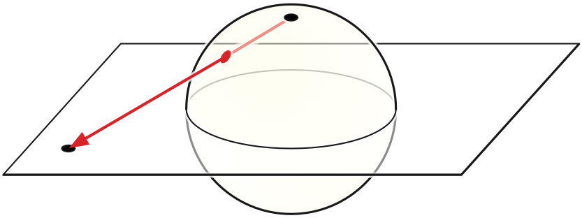
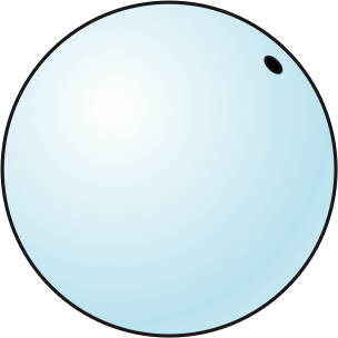
Formally, rotation systems (and their equivalent incidence lists) describe embeddings onto the sphere \(S^2 = \{ (x,y,z) \mid x^2+y^2+z^2=1 \}\), not onto the plane. Indeed, for many results about planar graphs, it is actually more natural to consider spherical embeddings on the sphere instead the plane. Fortunately, we can transfer embeddings back and forth between the sphere and the plane using stereographic projection.
Stereographic projection is the function \(\textsf{st}\colon S^2\setminus(0,0,1) \to \mathbb{R}^2\) where \(\textsf{st}(x,y,z) := \big(\! \frac{x}{1-z}, \frac{y}{1-z} \!\big)\). The projection \(\textsf{st}(p)\) of any point \(p\in S^2\setminus(0,0,1)\) is the intersection of the line through \(p\) and the “north pole” \((0,0,1)\) with the \(xy\)-plane. Points in the northern hemisphere project outside the unit circle; points in the southern hemisphere project inside the unit circle. Given any spherical embedding, if we rotate the sphere so that the embedding avoids \((0,0,1)\), stereographic projection gives us a planar embedding; conversely, given any planar embedding, inverse stereographic projection immediately gives us a spherical embedding. Thus, a graph is planar if and only if it has an embedding on the sphere.
To fully specify an embedding on the plane using a rotation system, we must somehow also indicate which face of the embedding is the outer face, or equivalently, which face of the corresponding spherical embedding contains the north pole. The outer face can be chosen arbitrarily.
Most of the exposition in these notes implicitly considers only embeddings of graphs with at least one edge. Exactly one map violates this assumption, namely the trivial map, which has one vertex, one face, and no edges. The trivial map is represented by the empty rotation system \((\varnothing, \varnothing, \varnothing)\).
“There are dinner jackets and dinner jackets. This is the latter.”
— Vesper Lynd [Eva Green], Casino Royale (2006)
It is somewhat confusing standard practice to use the same symbol \(G\) (and the same word “graph”) to simultaneously denote at least six formally different structures:
Even when authors do distinguish between graphs and maps, it is standard practice to conflate abstract graphs, the corresponding topological graphs, and images of embeddings as “graphs”. In particular, the image of a planar graph embedding is commonly called a plane graph. Even the phrases “abstract graph” and “topological graph” are non-standard; the standard names for these objects are “graph” (spoken by a combinatorialist) and “graph” (spoken by a topologist), respectively.7 It is also standard practice to use the word “embedding” to mean both an injective function from \(G^\top\) to the plane and the image of such a function, and to use the word “map” to mean both the decomposition of the plane induced by an embedding and the rotation system of that embedding.
I will try to carefully distinguish between these various objects when the distinction matters, but there is a serious tension here between formality and clarity, so I am very likely to slip occasionally.
Recall that a combinatorial map is a triple \(\Sigma = (D, \textsf{rev}, \textsf{succ})\), where \(D\) is a set of darts, is an involution of \(D\), and is a permutation of \(D\). For any such triple, the triple \(\Sigma^* = (D, \textsf{rev}, \textsf{rev}\circ\textsf{succ})\) is also a well-defined combinatorial map, called the dual map of \(\Sigma\).8
In other words, each vertex \(v\), edge \(e\), dart \(d\), or face \(f\) of the original map \(\Sigma\) corresponds to—or more evocatively, “is dual to”—or more formally, IS—a face \(v^*\), edge \(e^*\), dart \(d^*\), or vertex \(f^*\) of the dual map \(\Sigma^*\), respectively.
The endpoints of any primal edge \(e\) are dual to the shores of the corresponding dual edge \(e^*\), and vice versa. Specifically, for any dart \(d\), we have \(\textsf{head}(d^*) = \textsf{left}(d)^*\) and \(\textsf{tail}(d^*) = \textsf{right}(d)^*\). Intuitively, the dual of a dart is obtained by rotating it a quarter-turn counterclockwise.
Duality is trivially an involution: \((\Sigma^*)^* = \Sigma\), because \(\textsf{rev}\circ\textsf{rev}\circ\textsf{succ} = \textsf{succ}\). It immediately follows that for any dart \(d\), we have \(\textsf{left}(d^*) = \textsf{head}(d)^*\) and \(\textsf{right}(d^*) = \textsf{tail}(d)^*\).
We can also directly define the dual of a topological map \(\Sigma\) as follows. Choose an arbitrary point \(f^*\) in the interior of each face \(f\) of \(\Sigma\). Let \(F^*\) denote the collection of all such points. For each edge \(e\) of \(\Sigma\), choose a simple path \(e^*\) between the chosen points in the shores of \(e\), such that \(e^*\) intersects \(e\) once transversely and does not intersect any other edge of \(\Sigma\). Let \(E^*\) denote the collection of all such paths. These paths partition the plane into regions \(V^*\), each of which contains a unique vertex.9 The dual map \(\Sigma^*\) is the decomposition of the plane into vertices \(F^*\), edges \(E^*\), and faces \(V^*\).
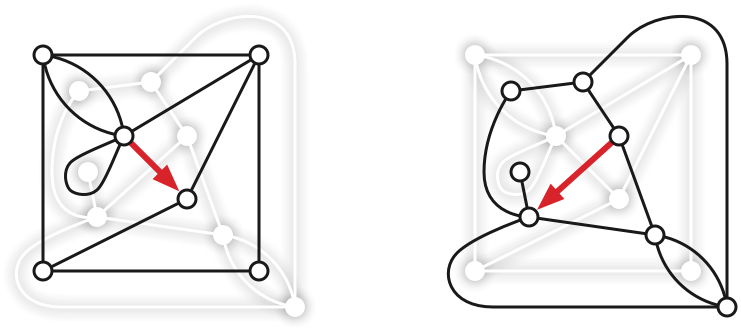
[[ add dual navigation figure ]]
When \(G\) is an embedded graph, it is extremely common to define the dual graph \(G^*\) as the 1-skeleton of the dual map of the embedding. This habit is a bit misleading, however; duality is a correspondence between maps or embeddings, not between abstract graphs. An abstract planar graph can have many non-isomorphic planar embeddings, each of which defines a different “dual graph”. Moreover, the dual of a simple embedded graph is not necessary simple; any vertex of degree \(2\) in \(G\) gives rise to parallel edges in \(G^*\), and any bridge in \(G\) is dual to a loop in \(G^*\). This is why we don’t want graphs to be simple by definition!
[[Duality is not a transformation; it’s just a type-cast]]
| Primal \(\Sigma\) | Dual \(\Sigma^*\) | Primal \(\Sigma\) | Dual \(\Sigma^*\) |
|---|---|---|---|
| vertex \(v\) | face \(v^*\) | \(\textsf{head}(d)\) | \(\textsf{left}(d^*)\) |
| dart \(d\) | dart \(d^*\) | \(\textsf{tail}(d)\) | \(\textsf{right}(d^*)\) |
| edge \(e\) | edge \(e^*\) | \(\textsf{left}(d)\) | \(\textsf{head}(d^*)\) |
| face \(f\) | vertex \(f^*\) | \(\textsf{right}(d)\) | \(\textsf{tail}(d^*)\) |
| \(\textsf{succ}\) | \(\textsf{rev}\circ\textsf{succ}\) | clockwise | counterclockwise |
| \(\textsf{rev}\) | \(\textsf{rev}\) |
There are several apparently arbitrary choices to make in the definitions of incidence lists, rotation systems, and duality. Should we store cycles of darts with the same head or the same tail? Should darts be ordered in clockwise or counterclockwise order around vertices? Or around faces? Should \(\textsf{head}(d^*)\) be defined as \(\textsf{left}(d)^*\) or \(\textsf{right}(d)^*\)? Different standards are used by different authors, by the same authors in different papers, and sometimes even within the same paper.10 (Mea culpa!)
Let me attempt to justify, motivate, or at least provide mnemonics for the specific choices I use in these notes. Some of these rules will only make sense later.
This standard creates an annoying discrepancy between the mathematical abstraction of a rotation system and its implementation as an incidence list. Rotation systems order darts around their heads because that makes the math cleaner, but incidence lists (typically) order darts around their tails because that better fits our intuition about searching graphs by following directed edges outward. Rather than give up either useful intuition, we’ll rely on (and if necessary implement) the identity \(\textsf{next}(d) = \textsf{rev}(\textsf{succ}(\textsf{rev}(d)))\).
Let \(\Sigma = (V, E, F)\) be an arbitrary planar map. In addition to the dual map \(\Sigma^*\), there are several other useful maps that can be derived from \(\Sigma\) in terms of two local features.
A flag of \(\Sigma\) is a vertex-edge-face triple \((v,e,f)\) such that \(v\) is an endpoint of \(e\) and \(f\) is a shore of \(e\).
A corner of \(\Sigma\) is a pair of flags that share the same vertex and the same face. Intuitively, a corner is an incidence between a vertex and a face, or if you prefer, a pair of edges whose darts are consecutive around a vertex, or around a face. (Formally, a corner is just a nickname for a dart; for each dart \(d\), the corresponding corner is the incidence between the vertex \(\textsf{head}(d)\) and the face \(\textsf{left}(d)\), or equivalently, between the vertex \(\textsf{tail}(\textsf{succ}^*(d))\) and the face \(\textsf{right}(\textsf{succ}(d))\).)
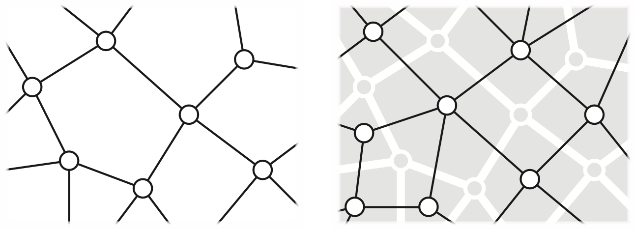
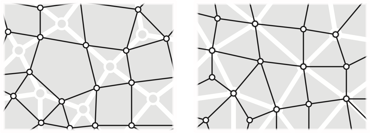
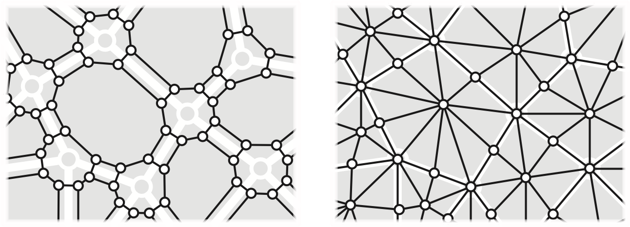
The medial map \(\Sigma^\times = (E, C, V\cup F)\) is the map whose vertices correspond to the edges of \(\Sigma\), whose edges correspond to the corners of \(\Sigma\), and whose faces correspond to vertices and faces of \(\Sigma\). The medial map of \(\Sigma\) is the image graph of a generic planar multicurve. Specifically, two vertices are connected by an edge in \(\Sigma^\times\) if the corresponding edges in \(\Sigma\) are adjacent in cyclic order around any vertex (or equivalently, around any face). Every map \(\Sigma\) and its dual \(\Sigma^*\) share the same medial map \(\Sigma^\times\).
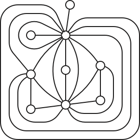
The dual of the medial map is called the radial map \(\Sigma^\diamond = (V\cup F, C, E)\). The radial map can be constructed from \(\Sigma\) by placing a new vertex in the interior of each face \(f\) of \(\Sigma\), connecting each face-vertex \(f\) to each vertex incident to \(f\) (with the appropriate multiplicity), and then erasing the original edges. Thus, each edge of \(\Sigma\) becomes a quadrilateral face of \(\Sigma^\diamond\). Again, every map \(\Sigma\) and its dual \(\Sigma^*\) share the same radial map \(\Sigma^\diamond\).
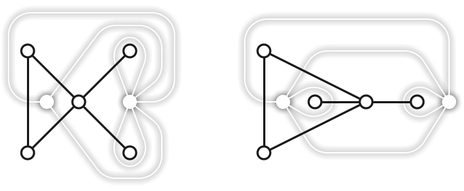
The band decomposition or ribbon decomposition of \(\Sigma\) is a map \(\Sigma^\square\) whose vertices correspond to the flags of \(\Sigma\). Two flags define an edge in \(\Sigma^\square\) if they differ in exactly one component: the same vertex and edge but a different face, the same vertex and face but a different edge, or the sane edge and face bu a different vertex. Every vertex of \(\Sigma^\square\) has degree \(3\). The faces of \(\Sigma^\square\) correspond to the vertices, edges, and faces of \(\Sigma\). Every map \(\Sigma\) and its dual \(\Sigma^*\) share the same band decomposition \(\Sigma^\square\).
The dual of the band decomposition is the barycentric subdivision \(\Sigma^+\). This map can be constructed by adding a new vertex in the interior of each edge, subdividing it into two edges, adding a new vertex in the interior of every face, and finally connecting each face-vertex to its vertices and edge midpoints. Thus, the vertices of \(\Sigma^+\) correspond to the vertices, edges, and faces of \(\Sigma\), and the faces of \(\Sigma^+\) correspond to the flags of \(\Sigma\). Every face of \(\Sigma^+\) is a triangle. Again, every map \(\Sigma\) and its dual \(\Sigma^*\) share the same barycentric subdivision \(\Sigma^+\).
These four derived maps are formally well-defined if and only only if the original map \(\Sigma\) has at least one edge. It is sometimes convenient, for example in base cases of inductive arguments, to informally extend the definitions to the trivial map \(\bullet\) as follows:
The trivial medial map \(\bullet^\times\) and the trivial band decomposition \(\bullet^\square\) both consist of a single closed curve on the sphere, with no vertices and two faces, corresponding to the vertex and face of \(\bullet\). I recommend thinking of this object as the result of gluing two flat circular disks together around their boundary.
The trivial radial map \(\bullet^\diamond\) and the trivial barycentric subdivision \(\bullet^+\) both consist of a single “edge”, with no faces and two vertices, again corresponding to the vertex and face of \(\bullet\). I recommend thinking of this object as an infinitely thin cylinder with its ends pinched to points.
But let me emphasize that these extensions are informal; the objects I’ve just described are not maps at all!
Consider using more mnemonic \(\textsf{hnext}\) instead of \(\textsf{succ}\), and similar for other nearby darts:
Our definition of graphs allows graphs with infinitely (even uncountably) many vertices and edges, and in particular, vertices with infinite (even uncountable) degree. Most of the graphs we consider in this course are finite, and obviously algorithms can only explicitly construct finite graphs. However, we do sometimes implicitly represent infinite graphs with certain symmetries using finite graphs. For example, any triangulation of a polygon with holes (a finite planar map, whose dual is another planar map) is an implicit representation of its universal over (an infinite planar map whose dual is an infinite tree).↩︎
And again, the definition allows topological graphs with infinitely (even uncountably) many vertices and edges, and infinite (even uncountable) vertex degrees.↩︎
Even worse, graph theorists use the phrase “topological graph” to mean a generic drawing or immersion of a graph in the plane. In a generic drawing, vertices are represented by distinct points; edges are represented by paths between their endpoints; no edge passes through a vertex except its endpoints; all (self-)intersections between edge interiors are transverse; and all pairwise (self-)intersection points are distinct.↩︎
For readers familiar with topology, a triangulation is not necessarily a simplicial complex, but rather what Hatcher calls a \(\Delta\)-complex.↩︎
Because the edges of a planar embedding can be arbitrary paths, it is not immediately obvious that this cyclic order is well-defined. In fact, the existence of a consistent order follows from careful application of the Jordan-Schönflies theorem.↩︎
or into the sphere, or an isotopy/homeomorphism class of such embeddings↩︎
Even worse, graph theorists use the phrase “topological graph” to mean a generic drawing or immersion of a graph in the plane. In a generic drawing, vertices are represented by distinct points; edges are represented by paths between their endpoints; no edge passes through a vertex except its endpoints; all (self-)intersections between edge interiors are transverse; and all pairwise (self-)intersection points are distinct.↩︎
The dual rotation system of a planar map is sometimes also called a polygonal schema, because it describes how to construct the map from a collection of disjoint planar polygons (the faces) by identifying pairs of boundary edges.↩︎
You should verify this claim!↩︎
I can’t resist quoting Herodotus’ Histories, written around 440BCE: “The ordinary [Greek] practice at sea is to make sheets fast to ring-bolts fitted outboard; the Egyptians fit them inboard. The Greeks write and calculate from left to right; the Egyptians do the opposite. Yet they say that their way of writing is toward the right, and the Greek way toward the left.” Herodotus was strangely silent on which end of the egg the Egyptians ate first, or whether they preferred to fight a hundred duck-sized horses or one horse-sized duck.↩︎