Maxwell–Cremona Correspondence

The idea of using graphs to model physical networks of springs or ropes under tension does not originate with Tutte, but centuries earlier.

In the late 1500s, the Dutch physicist Simon Stevin published an influential book called The Art of Weighing. The 1605 reissue of this book included a supplement where Stevin describes how to calculate the forces imposed by a weight hanging from a tree of ropes. In particular, Stevin correctly observes that as long as every vertex of this tree has degree \(3\), there is a unique force applied along each rope such that all forces balance out.

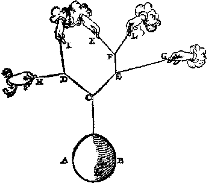
More than a century later, the French engineer Pierre Varignon described a method for visualising the forces acting on a planar tree of ropes under tension. The network of ropes is sometimes called a funicular polygon, from the Latin funiculus meaning “small rope”, and the Greek polygonos meaning “many-angled”. (It would be another 45 years before Meister redefined “polygon” to mean a closed curve composed of line segments.

Each edge in the funicular polygon is a line segment. We can visualize the forces acting along these edges by drawing a force polygon as follows. For each edge \(e\) in the funicular polygon, we draw a line segment \(e^*\) perpendicular¹ to \(e\) whose length is equal to the magnitude of force being applied along \(e\). If the system of ropes is in equilibrium, then the forces vectors into each vertex of the funicular polygon sum to zero; equivalently, the corresponding edges of the force polygon form a closed figure. In short, the force polygon is the dual graph of the funicular polygon. Outside the study of polyhedra (and especially regular polyhedra), this may be the oldest example of planar-graph duality.²

Finally, in the mid-1800s, famed Scottish physicist James Clark Maxwell generalized Varignon’s force diagrams to arbitrarily complex planar graphs. Maxwell’s analysis became a key technique in the new field of graphical statics developed by William John Macquorn Rankine, Carl Culmann, Luigi Cremona, and others. One of the early successes of graphical statics was the world’s tallest man-made structure (at the time), constructed in the 1880s to celebrate the 100-year anniversary of the French Revolution by Gustave Eiffel.

Dramatis Personae

Graphs and Frameworks

Let \(G\) be a simple 3-connected planar graph. Recall from the previous lecture that \(G\) has a unique planar embedding (up to homeomorphism) and therefore has a unique dual graph \(G^*\), which is also simple, 3-connected, and planar.

Let \(\langle uv | ab\rangle\) denote the unique dart \(d\) in \(G\) with tail \(u\) and head \(v\), whose dual dart \(d^*\) in \(G^*\) has tail \(a\) and head \(b\). Thus, \(\langle uv | ab \rangle^* = \langle ab | uv \rangle\) and \(\textsf{rev} \langle uv | ab \rangle = \langle vu | ba \rangle\). Equivalently, \(\langle uv | ab \rangle\) has right shore \(a^*\) and left shore \(b^*\) in the unique planar embedding of \(G\).

A position function for \(G\) is a function \(p\colon V(G)\to\mathbb{R}^2\), or equivalently a matrix \(p\in (\mathbb{R}^2)^n = \mathbb{R}^{2\times n}\), such that \(p(u)\ne p(v)\) for every edge \(uv\). For each edge \(uv\) of \(G\), we abuse notation by writing \(p(uv)\) to denote the straight line segment between \(p(u)\) and \(p(v)\). The pair \((G, p)\) is called a planar framework. The displacement vector \(\Delta(d)\) of any dart \(d = \langle uv | ab \rangle\), with respect to a fixed position function \(p\), is \(p(v) - p(u)\).

Let me emphasize that a planar framework \((G,p)\) is a straight-line drawing of its underlying planar graph \(G\), but it is not necessarily an embedding; images of distinct edges may cross, overlap, or even coincide.

Stresses

A stress is a function \(\omega\colon E(G)\to\mathbb{R}\), or equivalently, a vector \(\omega\in \mathbb{R}^m\). A stress is non-zero if \(\omega(e)\ne 0\) for at least one edge \(e\), and strict if \(\omega(e)\ne 0\) for every edge \(e\). We frequently abuse notation by defining \(\omega(uv)=0\) when \(uv\) is not an edge. We also extend the function \(\omega\) to the darts of \(G\) by defining \(\omega(\langle uv | ab \rangle) = \omega(uv)\).

We can interpret each edge \(e\) of a planar framework as a (first-order linear) spring with spring constant \(|\omega(e)|\), under tension if \(\omega(e)>0\) and under compression if \(\omega(e)<0\). Hooke’s Law implies that each edge \(uv\) imparts a force of \(\omega(uv) \cdot (p(v) - p(u)) = \omega(uv)\cdot \Delta(u\mathord\to v)\) to vertex \(v\).

A stress \(\omega\) is called an equilibrium stress (or a self-stress) if the net force on every vertex is zero; that is, for every vertex \(v\) we have \[ \sum_u \omega(uv) \cdot (p(v) - p(u)) = \binom{0}{0}\]

Recall from the previous lecture that this linear system describes the unique critical point of the potential energy function \[ \Phi(p) := \frac{1}{2} \sum_{u, v} \omega(uv) \cdot \| p(u) - p(v) \|^2. \] Because stress coefficients are allowed to be negative, this unique critical point is no longer a local minimum, as it was in the previous lecture.

1-Forms and Discrete Integration

A discrete 1-form (or 1-cochain, or voltage assignment, or pseudoflow) on \(G\) is an anti-symmetric function \(\phi\colon D(G) \to R\) from the darts of \(G\) to some additive abelian group \(R\), where anti-symmetry means \(\phi(d) = -\phi(\textsf{rev}(d))\) for every dart \(d\). Here we consider only 1-chains over the vector spaces \(\mathbb{R}\) and \(\mathbb{R}^2\). (Let me emphasize here that a stress is not a 1-form!)

A 1-form is exact if the sum of the values of the darts in any directed cycle is zero. Exact 1-forms are also called tensions; they are also said to obey Kirchhoff’s voltage law.³

A vertex potential (or price function or discrete \(0\)-form) is any function \(\pi\colon V(G)\to R\) over the vertices of \(G\). The derivative (or coboundary) \(\delta\pi\) of a \(0\)-form \(\pi\) is the 1-form \(\delta\pi(u\mathord\to v) := \pi(v) - \pi(u)\).

Lemma: A 1-form \(\phi\) is exact if and only if \(\phi\) is the derivative of a vertex potential.

Proof:

The derivative \(\delta\pi\) of any \(0\)-form \(\pi\) is clearly exact. On the other hand, given any exact \(1\)-form \(\phi\), we can arbitrarily fix the potential \(\pi(o)\) of an arbitrary vertex \(o\), and then for any other vertex define \(\pi(v)\) by summing (or “integrating”) \(\phi\) along any path from \(o\) to \(v\). Exactness of \(\phi\) implies that \(\pi(v)\) does not depend on which path we choose to sum along. More generally, for any vertices \(s\) and \(t\), we can compute the potential difference \(\pi(t)-\pi(s)\) by “integrating” \(\phi\) along any \(s\)-to-\(t\) path.

In particular, for any fixed planar framework \((G, p)\), the displacement function \(\Delta \colon D(G) \to \mathbb{R}^2\) defined by \(\Delta(u\mathord\to v) = p(v) - p(u)\) is an exact 1-form.

A 1-form over a 3-connected planar graph (or more generally, any surface map) is closed if the sum of the values of the darts in any face boundary of \(G\) sum to zero. Exact 1-forms are also called cocirculations.

Lemma:

Let \(G\) be an arbitrary 3-connected planar graph. A 1-form on \(G\) is closed if and only if it is exact.

Proof:

Every face boundary in \(G\) is a directed cycle by definition, so every exact 1-form is trivially closed (even if the graph \(G\) is not planar). The Jordan curve theorem applied to any planar embedding of \(G\) implies that every directed cycle in \(G\) is a sum (or symmetric difference) of directed face boundaries. \(\qquad\square\)

Reciprocal diagrams

A reciprocal diagram for a planar framework \((G, p)\) is another planar framework \((G^*, p^*)\) such that \(G^*\) and \(G\) are dual and corresponding edges in \(G\) and \(G^*\) are mapped to orthogonal segments by \(p\) and \(p^*\), respectively. Two reciprocal diagrams are equivalent if one is a translation of the other. For any vector \(v\in \mathbb{R}^2\), let \(v^\perp\) denote the result of rotating \(v\) a quarter turn counterclockwise: \(\binom{x}{y}^\perp = \binom{-y}{x}\).

Theorem [Maxwell, Whiteley]:

There is a bijection between equilibrium stresses \(\omega\) for \((G, p)\) and equivalence classes of reciprocal diagrams \((G^*, p^*)\). Moreover, the stress \(\omega^*(e) = 1/\omega(e)\) is an equilibrium stress for every reciprocal diagram \((G^*, p^*)\), and the corresponding equivalence class of reciprocal diagrams of any \((G^*, p^*)\) contains \((G,p)\).

Proof:

Let \(\omega\) be any equilibrium stress for \((G,p)\). Define a 1-form \(\Delta^*\colon D(G^*)\to\mathbb{R}^2\), which might be called the dual displacement function, by setting \[ \Delta^*(d^*) := \omega(d)\cdot \Delta(d)^\perp \] for every dart \(d\) of \(G\). For any face \(v^*\) of the dual graph \(G^*\), equilibrium implies that \[\begin{aligned} \sum_{d^* \colon v^* = \textsf{left}(d^*)} \Delta^*(d^*) &= \sum_{d \colon v = \textsf{head}(d)} \omega(d)\cdot\Delta(d)^\perp \\ &= \sum_{u} \omega(uv) \cdot \Delta(u\mathord\to v)^\perp = \binom{0}{0}^\perp = \binom{0}{0}. \end{aligned}\] Thus, the function \(\Delta^*\) is a closed 1-form in the dual graph \(G^*\). , it follows that \(\Delta^*\) is an exact 1-form on \(G^*\). Thus, there is a potential function \(p^*\) on the vertices of \(G^*\) such that \(\Delta^*(a\mathord\to b) = p^*(b) - p^*(a)\) for all dual darts \(a\mathord\to b\); moreover, \(p^*\) is unique up to translation. By construction, the framework \((G^*, p^*)\) is a reciprocal diagram of \((G,p)\).

On the other hand, let \((G^*, p^*)\) be any reciprocal diagram for \((G,p)\). For each dart \(d = \langle uv | ab \rangle\), there is a unique real number \(\omega(d)\) such that \[ p^*(b) - p^*(a) = \omega(d) \cdot ( p(v) - p(u) )^\perp. \] Kirchoff’s voltage law in \((G^*, p^*)\) immediately implies that \(\omega\) is an equilibrium stress for \((G, p)\). \(\qquad\square\)

Polyhedral lifts

A lift of a planar framework \((G,p)\) is another height function \(z\colon V(G)\to\mathbb{R}\), or equivalently, a vector \(z\in \mathbb{R}^n\). The position and height functions define a three-dimensional position function \(\hat{p}\colon V(G)\to \mathbb{R}^3\) by concatenation: \(\hat{p}(v) = (x(v), y(v), z(v))\), where \((x(v), y(v)) = p(v)\). A lift of \((G,p)\) is polyhedral if, for each face \(f\) of \(G\), the images \(\hat{p}(v)\) of all vertices \(v\in f\) are coplanar; a polyhedral lift is trivial if all points \(\hat{p}(v)\) are coplanar. Finally, two polyhedral lifts \(z\) and \(z’\) are equivalent if their difference a constant: \(z(u) - z’(u) = z(v) - z’(v)\) for all vertices \(u\) and \(v\). For example, every trivial lift is equivalent to the zero lift \(h\equiv 0\).

Theorem [Maxwell, Whiteley]:

There is a bijection between reciprocal diagrams \((G^*, p^*)\) of \((G,p)\) and equivalence classes of nontrivial polyhedral lifts of \((G,p)\).

Proof:

The radial graph \(G^\diamond\) of \(G\) is a bipartite planar graph whose vertices correspond to the vertices and faces of \(G\), and whose edges correspond to vertex-face incidences or corners of \(G\). The radial graph \(G^\diamond\) inherits a unique planar embedding from the unique embeddings of \(G\) and \(G^*\). The faces of this embedding are correspond to the edges of \(G\); in particular, every face of \(G^\diamond\) has degree \(4\).⁴

Let \(z\) be any non-trivial polyhedral lift of \((G,p)\). For each face \(f\) of \(G\), let the equation \(z = x^*(f)\cdot x + y^*(f)\cdot y - z^*(f)\) denote the plane supporting the lifted face \(\hat{p}(f)\), and define \(p^*(f) = (x^*(f), y^*(f))\). For every corner \((v, f)\) in \(G\) (or equivalently, every edge \(vf\) of the radial map \(G^\diamond\)) we immediately have \[ z(v) + z^*(f) ~=~ x^*(f)\cdot x(v) + y^*(f)\cdot y(v) ~=~ p(v) \cdot p^*(f) \] Thus, for every dart \(d = \langle uv | ab \rangle\) of \(G\), we have four identities: \[ \begin{aligned} p(u)\cdot p^*(a) &= z(u) + z^*(a) \\ p(u)\cdot p^*(b) &= z(u) + z^*(b) \\ p(v)\cdot p^*(a) &= z(v) + z^*(a) \\ p(v)\cdot p^*(b) &= z(v) + z^*(b) \end{aligned} \] It follows that \((p(u)-p(v))\cdot(p^*(a)-p^*(b)) = 0\). We conclude that each edge of \((G,p)\) is orthogonal to its dual edge in \((G^*, p^*)\).

On the other hand, let \((G^*, p^*)\) be any reciprocal diagram for \((G,p)\). For each face \(f\) of \(G\) we interpret the dual position vector \(p^*(f)\) as the gradient vector \((x^*(f), y^*(f))\) of the support plane of the lifted face \(\hat{p}(f)\). We simultaneously compute vertical offsets \(z^*(f)\) for those support planes and heights \(z(v)\) for the vertices to obtain a consistent polyhedral lift.

We can assign values \(z(v)\) and \(z^*(f)\) to the vertices \(v\) and faces \(f\) of \(G\) by integrating a closed \(1\)-form over the darts of the radial map \(G^\diamond\). Specifically, we define the 1-form \(\phi^\diamond\colon D(G^\diamond)\to\mathbb{R}\) by setting \[\phi^\diamond(f\mathord\to v) := p(v)\cdot p^*(f),\] and therefore \[\phi^\diamond(v\mathord\to f) = -p(v)\cdot p^*(f),\] for each vertex \(v\) and face \(f\) of \(G\). For each dart \(d = \langle uv | ab \rangle\) of \(G\), reciprocality implies \[ \begin{aligned} \phi^\diamond(a\mathord\to v) + \phi^\diamond(v\mathord\to b) &{} + \phi^\diamond(b\mathord\to u) + \phi^\diamond(u\mathord\to a) \\ &= p(v)\cdot p^*(a) - p(v)\cdot p^*(b) + p(u)\cdot p^*(b) - p(u)\cdot p^*(a) \\ &= (p(v)-p(u)) \cdot (p^*(a) - p^*(b)) = 0. \end{aligned} \] Thus, \(\phi^\diamond\) is a closed, and therefore exact, 1-form on the radial graph \(G^\diamond\). It follows that there is a 0-form \(\pi^\diamond\colon V(G^\diamond) \to\mathbb{R}\), unique up to translation, such that \(\phi^\diamond(f\mathord\to v) = \pi^\diamond(v) - \pi^\diamond(f)\). For each vertex \(v\) of \(G\), define \(z(v) := \pi^\diamond(v)\), and for each face \(f\) of \(G\), define \(z^*(f) := -\pi^\diamond(f)\). By construction, for any corner \((v, f)\) of \(G\), we have \[ z(v) + z^*(f) = p(v)\cdot p^*(f) \] and therefore \[ z(v) = x(v)\cdot x^*(f) + y(v)\cdot y^*(f) - z^*(f). \] Thus, the point \(\hat{p}(v) = (x(v), y(v), z(v))\) lies on the supporting plane of \(\hat{p}(f)\), which has equation \(z = x^*(f)\cdot f + y^*(f)\cdot y - z^*(f)\). We conclude that the vertex heights \(z(v)\) and facet-plane offsets \(z^*(f)\) are consistent with a polyhedral lift of \(G\). \(\qquad\square\)

A Non-Obvious Example: The “Anticube”

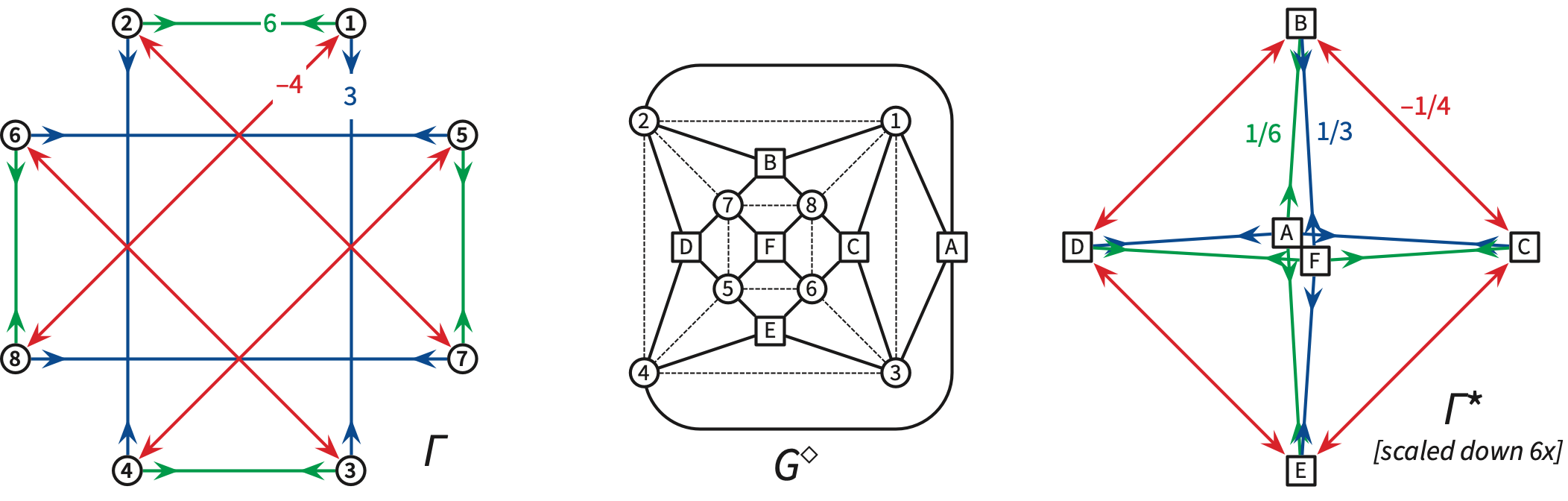
Consider the planar framework \(\Gamma = (G,p)\) shown below left, whose underlying graph \(G\) is the standard cube graph, which is planar and 3-connected. The six faces of the cube have vertices \(1243\), \(1276\), \(2457\), \(4365\), \(3186\), and \(5687\). (Short orthogonal edges have stress coefficient \(6\); long orthogonal edges have stress coefficient \(3\); diagonal edges have stress coefficient \(-4\).)

The resulting reciprocal framework \(\Gamma^* = (G^*, p^*)\) is shown on the right, scaled down by a factor of \(6\), along with its dual equilibrium stress. (Dual vertices \(A\) and \(F\) actually coincide, but are perturbed apart to better illustrate the framework structure.) The dual graph \(G^*\) is the graph of the regular octahedron. I computed this reciprocal framework by solving the system of linear equations \(\Delta^*(a\mathord\to b) = p^*(b) - p^*(a)\), one for each dual edge, for the dual position vectors \(p^*(a)\).

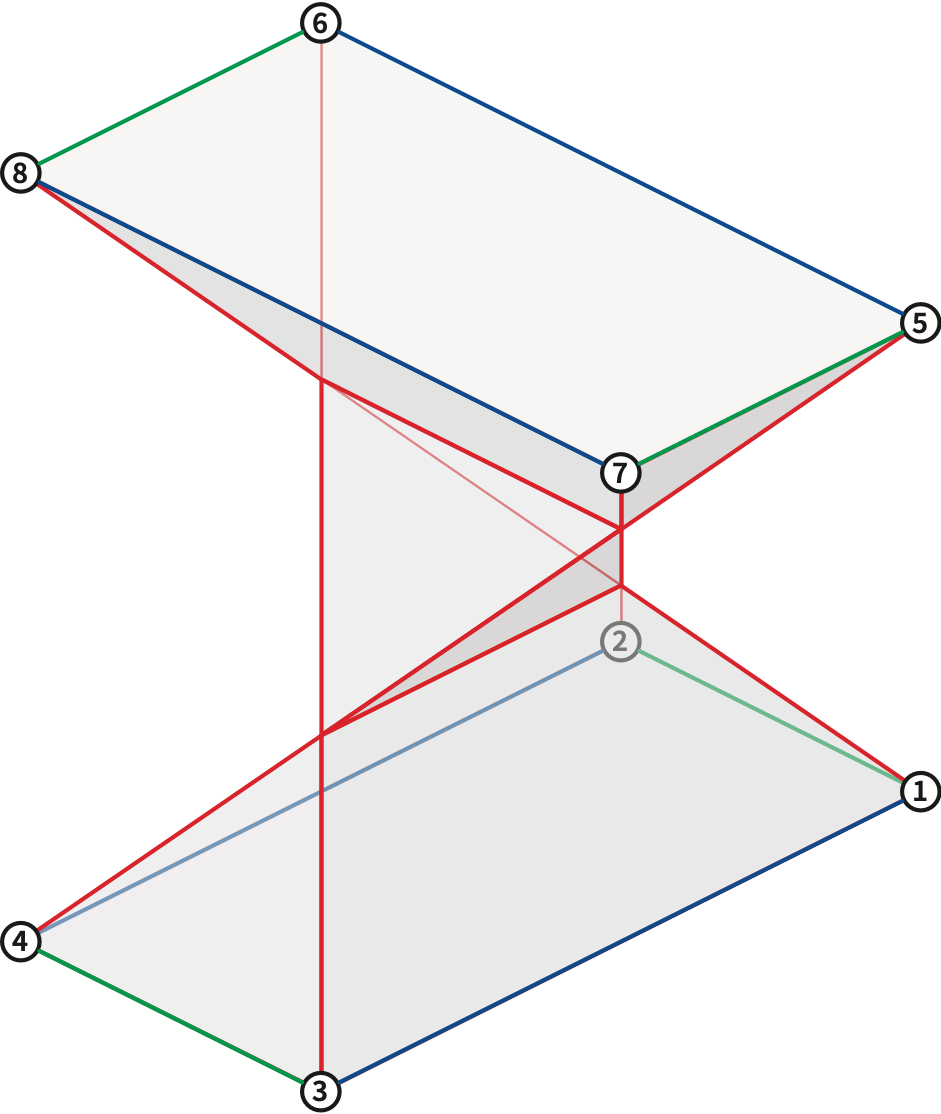
The next figure shows the polyhedral lift of the anticube corresponding to the given equilibrium stress (scaled vertically by a factor of \(9\)). This polyhedron appears to consist of two triangular prisms and a tetrahedron, but in fact it is a self-intersecting embedding of the cube; the corners of the central tetrahedron are not actually vertices of the polyhedron. Four of the six cube faces are embedded as planar but self-intersecting quadrilaterals; opposite pairs of these faces intersect each other. Again, I computed this polyhedral lift by solving the system of linear equations \(\phi^\diamond(f\mathord\to v) = \pi^\diamond(v) - \pi^\diamond(f)\), one for each radial edge, for the radial vertex potentials \(z(v) = \pi^\diamond(v)\) and \(z^*(f^*) = \pi^\diamond(f)\).

Steinitz’s Theorem

[[Write this!]]

For embedded planar frameworks, positive-stress bars lift to locally convex edges, and negative-stress bars lift to locally concave edges. We can solve for negative boundary stresses that turn any Tutte drawing into an self-stressed planar framework. The Maxwell–Cremona lift of the resulting framework is (the boundary of) a convex polytope.

Steinitz’s Theorem: Every 3-connected planar graph is the 1-skeleton of am essentially unique convex polytope in \(\mathbb{R}^3\).

(In fact, Steinitz only proved that every polyhedral planar map is equivalent to the boundary map of a convex polytope. Steinitz proved this theorem using a direct inductive construction via the medial map. The equivalence of 3-connected planar graphs and polyhedral embeddings was later proved by Whitney.)

Positive interior stresses lift to convex edges; negative interior stresses lift to concave edges.

We can’t actually solve for negative boundary stresses for arbitrary outer faces, but we can for triangles. Every simple planar map has either a face or a vertex of degree 3.

Non-3-connected Frameworks

The definitions of planar framework and equilibrium stress do not actually require the underlying graph to be planar and 3-connected. A planar framework is a pair \((G,p)\) where \(G\) is an arbitrary graph and \(p\colon V(G)\to\mathbb{R}^2\) is a position function for the vertices of \(G\). The adjective “planar” refers to the target space of the position function \(p\), not a the underlying graph of the framework. Similarly, the definition of equilibrium stress has nothing to do with the planarity or connectedness of the underlying graph.

If the underlying graph \(G\) of a planar framework \((G,p)\) is planar but not 3-connected, we no longer have a bijection between equilibrium stresses and equivalence classes of reciprocal diagrams. Instead, each planar embedding of \(G\) yields a different bijection between equilibrium stresses and reciprocal diagrams. In short, reciprocal diagrams are defined for planar embeddings, not just for abstract graphs.

The following figure shows a planar framework whose underlying graph two different planar embeddings, obtained by swapping the two “interior” vertices; the shaded green polygons indicate one face of each embedding. Each embedding yields a different reciprocal diagram for the same equilibrium stress. (The arrows indicate the rotation system around the vertex of the reciprocal diagram dual to the shaded green face in the primal framework.)

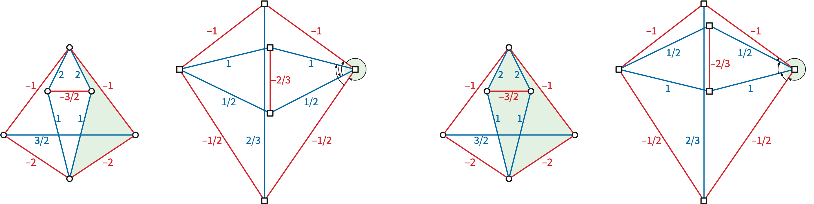
Each embedding similarly yields a different polyhedral lift of the framework \((G,p)\). One embedding is a tetrahedron with a notch carved out of one edge; the other is a self-intersecting polyhedron with convex faces that looks like two tetrahedra sharing an edge.

Non-Planar Frameworks

What about non-planar graphs? Every rotation system for a graph \(G\) yields a well-defined dual graph \(G^*\). But if the rotation system for \(G\) does not define a planar map, we lose the equivalence between closed and exact 1-forms in the resulting dual graph \(G^*\). The equilibrium stress at each vertex of \(G\) still defines (up to translation) a planar polygon of forces for the corresponding face of \(G^*\), but these polygons no longer necessarily fit together consistently in the plane.

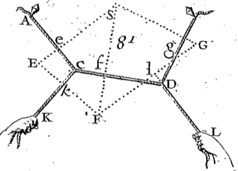
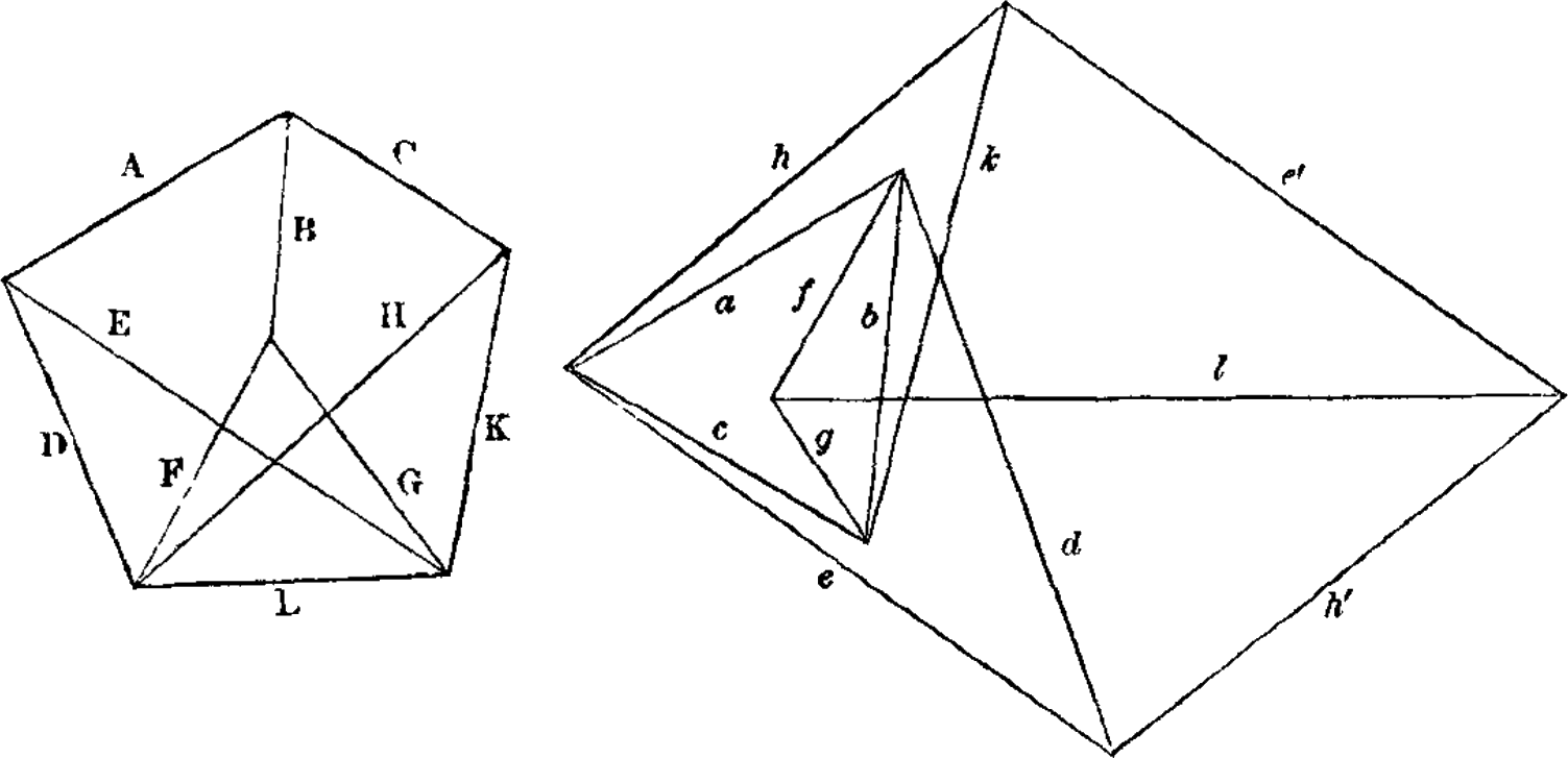
The final figures show two examples from Maxwell’s original papers. The first figure shows a framework on the left that has \(K_{3,3}\) as a subgraph and is therefore non-planar, together with an attempted reciprocal framework on the right. The framework on the left has two edges \(e\) and \(e'\) (respectively, \(h\) and \(h'\)) that are dual to the same edge \(E\) (respectively \(H\)) in the original framework, respectively. We can complete Maxwell’s construction by identifying these edge pairs, but the resulting structure no longer embeds in the plane; instead, we get a well-defined reciprocal framework in the flat torus!

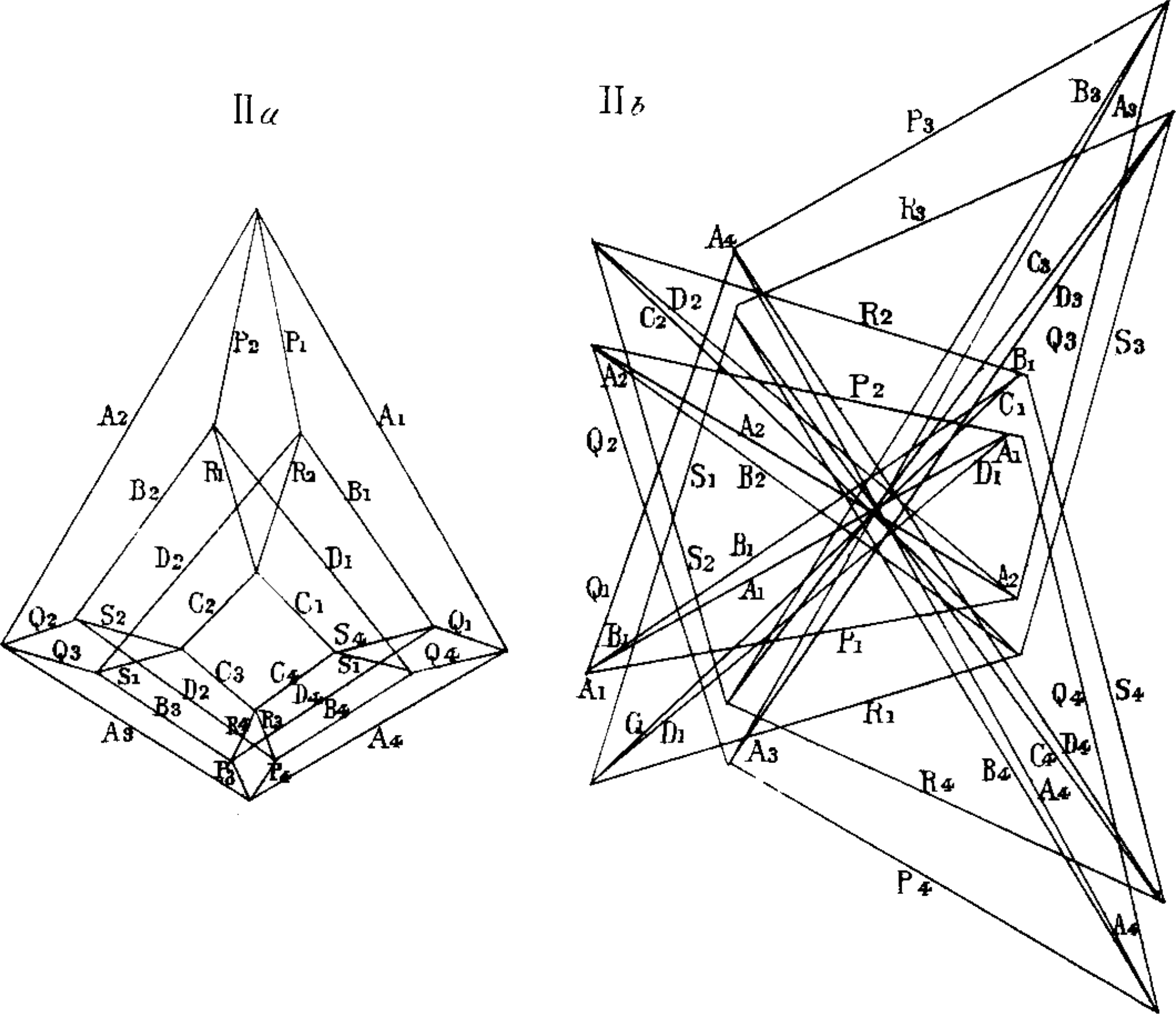
On the other hand, sometimes we get lucky. The last figure shows a planar framework \((G,p)\) whose underlying graph \(G\) is again not planar, but that has a natural embedding on the torus as a \(4\times 4\) toroidal grid. It’s fairly easy to construct an equilibrium stress for this framework by assigning positive stresses to one family of disjoint 4-cycles and negative stresses to the other family of disjoint 4-cycles. Maxwell constructs a reciprocal framework \((G^*, p^*)\) with respect to this toroidal embedding of \(G\) and such an equilibrium stress, and the result is a proper planar framework!

References

1. Henry Crapo and Walter Whiteley. Plane self stresses and projected polyhedra I: The basic pattern. Topologie structurale / Structural Topology 20:55–77, 1993.

2. Henry Crapo and Walter Whiteley. Spaces of stresses, projections and parallel drawings for spherical polyhedra. Beitr. Algebra Geom. 35(2):259–281, 1994.

3. Luigi Cremona. Le figure reciproche nella statica grafica. Tipografia di Giuseppe Bernardoni, 1872. English translation in [4].

4. Luigi Cremona. Graphical Statics. Oxford Univ. Press, 1890. English translation of [3] by Thomas Hudson Beare.

5. Eduard J. Dijksterhuis, editor. The Principal Works of Simon Stevin, Volume I. C. V. Swets & Zeitlinger, 1955. English translation by Carry Dikshoorn.

6. Peter Eades and Patrick Garvan. Drawing stressed planar graphs in three dimensions. Proc. 2nd Symp. Graph Drawing, 212–223, 1995. Lecture Notes Comput. Sci. 1027, Springer.

7. John E. Hopcroft and Peter J. Kahn. A paradigm for robust geometric algorithms. Algorithmica 7(1–6):339–380, 1992.

8. James Clerk Maxwell. On reciprocal figures and diagrams of forces. Phil. Mag. (Ser. 4) 27(182):250–261, 1864.

9. James Clerk Maxwell. On the application of the theory of reciprocal polar figures to the construction of diagrams of forces. Engineer 24:402, 1867. Reprinted in [109, pp. 313–316].

10. James Clerk Maxwell. On reciprocal figures, frames, and diagrams of forces. Trans. Royal Soc. Edinburgh 26(1):1–40, 1870.

11. James Clerk Maxwell. The Scientific Letters and Papers of James Clerk Maxwell. Volume 2: 1862–1873. Cambridge Univ. Press, 2009.

12. Ares Ribó Mor, Günter Rote, and André Schulz. Small grid embeddings of 3-polytopes. Discrete Comput. Geom. 45(1):65–87, 2011.

13. Ernst Steinitz. Polyeder und Raumeinteilungen. Enzyklopädie der mathematischen Wissenschaften mit Einschluss ihrer Anwendungen III.AB(12):1–139, 1916.

14. Ernst Steinitz and Hans Rademacher. Vorlesungen über die Theorie der Polyeder: unter Einschluß der Elemente der Topologie. Grundlehren der mathematischen Wissenschaften 41. Springer-Verlag, 1934. Reprinted 1976.

15. Simon Stevin. Byvough der Weeghconst [Supplement to the Art of Weighing]. 1605. Reprinted and translated into English in [5, pp. 525–607].

16. Pierre Varignon. Nouvelle mechanique ou statique, dont le projet fut donné en M.DC.LXXVII. Claude Jombert, Paris, 1725.

17. Walter Whiteley. Motion and stresses of projected polyhedra. Topologie structurale / Structural Topology 7:13–38, 1982.

Aptly Named

• Homological constraints for planar reciprocal frameworks
• Impossible figures (cohomology, linear programming)
• Resolving force loads [Rote and Schulz]
• Rigidity (via LP duality)