Multiple-Source Shortest Paths, Revisited

In a recent breakthrough, Das, Kipouridis, Probst Gutenberg, and Wulff-Nilsen described an alternative algorithm that solves the planar multiple-source shortest path problem using a relatively simple divide-and-conquer strategy. Their algorithm theoretically runs in \(O(n\log h)\) time, where \(h\) is the number of vertices on the outer face, which improves the \(O(n\log n)\) time of Klein’s algorithm when \(h\) is small. Moreover, this running time is worst-case optimal as a function of both \(n\) and \(h\).

A better expression for the running time is \(O(S(n)\log h)\), where \(S(n)\) is the time to compute a single-source shortest path tree.

• If we use Dijkstra’s algorithm off the shelf, the running time is \(O(n\log n \log h)\).
• If we use the \(O(n\log\log n)\)-time algorithm that we will see in Lecture 15,¹ the running time is \(O(n\log h\log\log n)\).
• If we use the \(O(n)\)-time algorithm of Henzinger et al.,² the running time is the optimal \(O(n\log h)\).

The new algorithm is simpler in the sense that it uses only black-box shortest-path algorithms, completely avoiding complex dynamic forest data structures that are inefficient in practice, at least for small graphs.³ On the other hand, the new algorithm requires a subtle divide-and-conquer algorithm with weighted \(r\)-divisions, which is also inefficient in practice, to achieve its best possible running time \(O(n\log h)\). On the gripping hand, Klein’s algorithm has been observed to require a sublinear number of pivots for many inputs, so the \(O(n\log n)\) time bound, while tight in the worst case, is usually conservative; whereas, the \(O(n\log h)\) time bound for the new algorithm is tight for all inputs. It would be interesting to experimentally compare Klein (or CCE) using linear-time dynamic trees against the new algorithm using Dijkstra as a black box.

Problem formulation

It will be convenient to describe the inputs and outputs of the MSSP problem slightly differently than in the previous lecture.

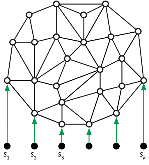
The input consists primarily of a directed planar map \(\Sigma = (V, E, F)\) with a distinguished outer face \(o\) and a non-negative weight \(\ell(u\mathord\to v)\) for every directed edge/dart \(u\mathord\to v\), which could be infinite (to indicate that a directed edge is missing from the graph). The weights are not necessarily symmetric; we allow \(\ell(u\mathord\to v) \ne \ell(v\mathord\to u)\).

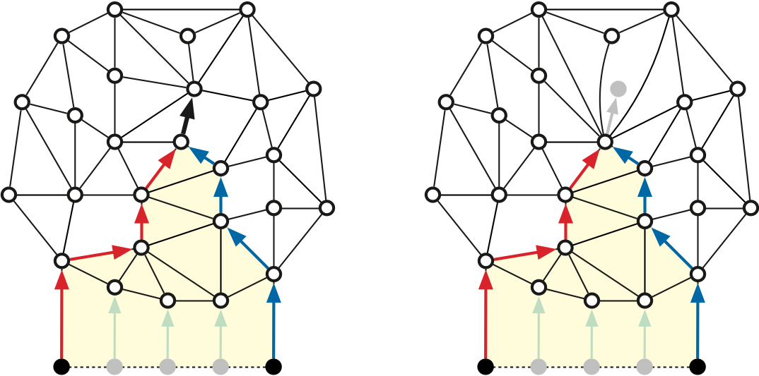
Let \(s_0, s_1, \dots, s_{h-1}\) be any subsequence of \(h\) vertices in counterclockwise order around the outer face, and let \(S = \{s_0, s_1, \dots, s_{h-1}\}\). Our goal is to compute an implicit representation of the shortest paths from each source \(s_i\) to every original vertex of \(\Sigma\). See Figure 1.

For ease of presentation, I will make a few minor technical assumptions:

• Every source vertex \(s_i\in S\) has out-degree \(1\) and in-degree \(0\). We can enforce this assumption if necessary by adding a new artificial source vertex \(s'_i\) and a single directed edge \(s'_i \mathord\to s_i\) with weight \(0\).
• \(\Sigma\) is simple. We can enforce this condition if necessary by resolving parallel edges and deleting loops in \(O(n)\) time using hashing.⁴
• The graph of \(\Sigma \setminus S\) is strongly connected. Thus, the shortest path tree rooted at each source vertex \(s_i\) includes every non-source vertex. We can enforce this assumption if necessary by adding new infinite-weight edges.
• All shortest paths are unique. If necessary, we can enforce this assumption either by randomly perturbing the edge weights or by choosing leftmost shortest paths, just as in the previous lecture.

For any index \(j\) and any vertex \(v\), let \(\mathit{path}_j(v)\) denote the shortest path in \(\Sigma\) from \(s_j\) to \(v\), let \(\mathit{dist}_j(v)\) denote the length of this shortest path, and let \(\mathit{pred}_j(v)\) denote the predecessor of \(v\) in this shortest path.

The main recursive algorithm \(\textsf{MSSP-Prep}\) preprocesses the map \(\Sigma\) into a data structure that implicitly encodes the single-source shortest path trees rooted at every source \(s_j\). A separate query algorithm \(\textsf{MSSP-Query}(s_j, v)\) returns \(\mathit{dist}_j(v)\).

Overview

The preprocessing algorithm uses a divide-and conquer-strategy. The input to each recursive call \(\textsf{MSSP-Prep}(H, i, k)\) consists of the following:

• A planar map \(H\), which is a simple weighted minor of the top-level input map \(\Sigma\).
• Two indices \(i\) and \(k\). To simplify presentation, we implicitly assume that \(s_i, s_{i+1}, \dots, s_k\) are the only source vertices in \(H\).

For each index \(j\), let \(T_j\) denote the tree of shortest paths in \(H\) from \(s_j\) to every other vertex of \(H\). The recursive call \(\textsf{MSSP-Prep}(H, i, k)\) computes an implicit representation of all \(k-i+1\) shortest path trees \(T_1, T_{i+1}, \dots, T_k\). The top-level call is \(\textsf{MSSP-Prep}(\Sigma, 0, h-1)\).

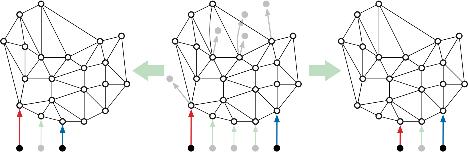
\(\textsf{MSSP-Prep}\) invokes a subroutine \(\textsf{Filter}(H, i, k)\) that behaves as follows:

• Compute the shortest path trees \(T_i\) and \(T_k\) rooted at \(s_i\) and \(s_k\).
• Identify directed edges that are shared by all shortest path trees \(T_j\) with \(i\le j\le k\).
• Contract shared edges and update nearby weights to maintain shortest path distances.
• Return the resulting contracted planar map.

Finally, ignoring base cases for now, \(\textsf{MSSP-Prep}(H,i,k)\) has four steps:

• Set \(H’ \gets \textsf{Filter}(H, i, k)\).
• Set \(j \gets \lfloor (i+k)/2 \rfloor\).
• Recursively call \(\textsf{MSSP-Prep}(H’, i, j)\).
• Recursively call \(\textsf{MSSP-Prep}(H’, j, k)\).

Finally, \(\textsf{MSSP-Prep}(H,i,k)\) returns a record storing the following information:

• the indices \(i\) and \(k\)
• data about each vertex in \(H\) computed by \(\textsf{Filter}\)
• pointers to the records returned by the recursive calls

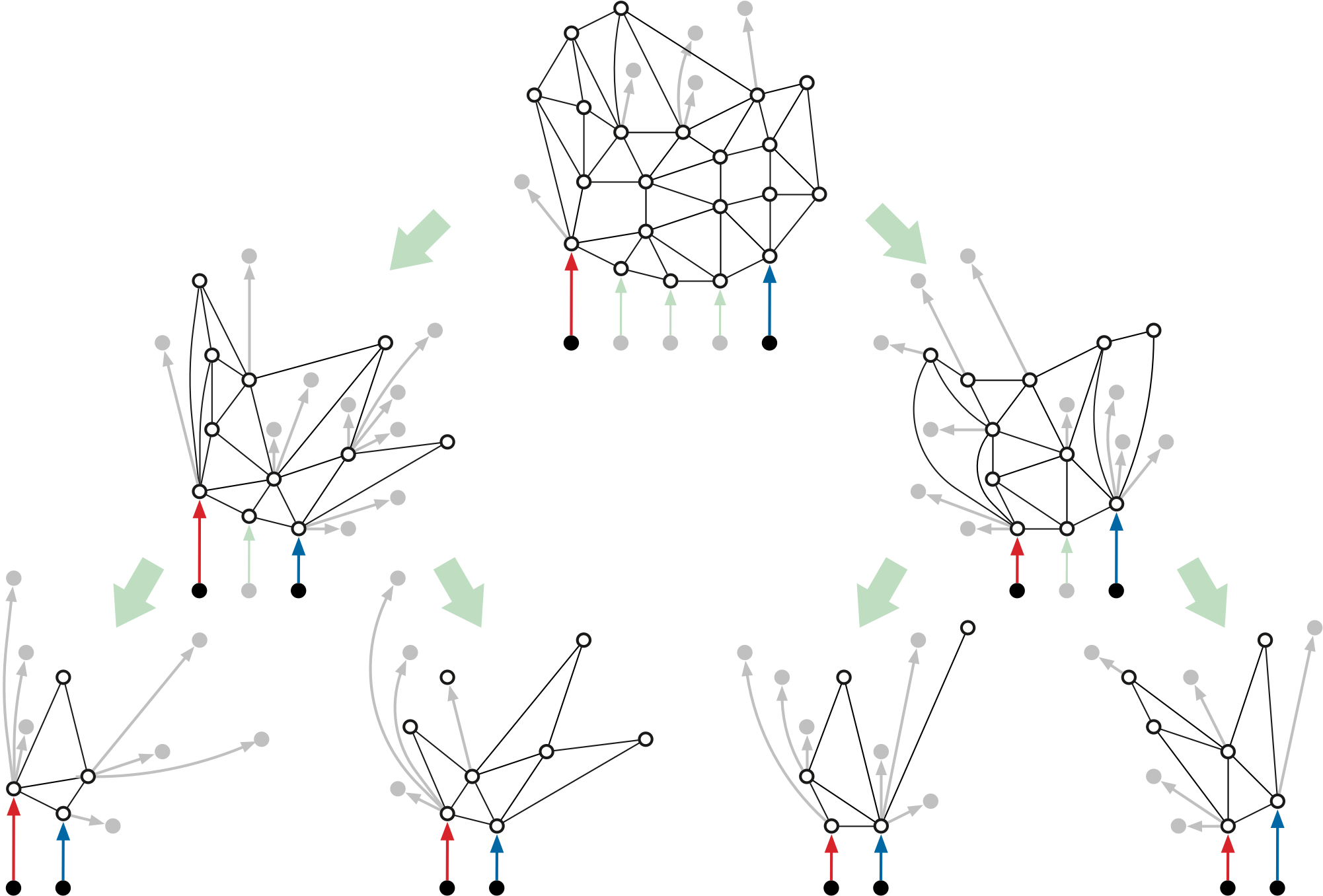
Said differently, \(\textsf{MSSP-Prep}\) returns a data structure that mirrors its binary recursion tree; every record in this data structure stores information computed by one invocation of \(\textsf{Filter}\).

The time and space analysis of \(\textsf{MSSP-Prep}\) hinges on the observation that the total size of all minors \(H\) at each level of the resulting recursion tree is only \(O(n)\). The depth of the recursion tree is \(O(\log h)\), so the total size of the data structure is \(O(n\log h)\). Similarly, aside from recursive calls, the time for each subproblem with \(m\) vertices is \(O(S(m))\), so the overall running time is \(O(S(n)\log h)\).

Finally, the query algorithm recovers the shortest-path distance from any source \(s_j\) to any vertex \(v\) by traversing the recursion tree of \(\textsf{MSSP-Prep}\) in \(O(\log h)\) time.

In the rest of this note, I’ll consider each of the component algorithms in more detail.

Properly shared edges

Now I’ll describe the filtering algorithm \(\textsf{Filter}(H, i, k)\) in more detail. For any index \(j\) and any vertex \(v\), define the following:

• \(T_j\) is the shortest-path tree in \(H\) rooted at source vertex \(s_j\).
• \(\mathit{dist}_j(v)\) is the shortest-path distance in \(H\) from \(s_j\) to \(v\).
• \(\mathit{pred}_j(v)\) is the predecessor of \(v\) on the shortest path in \(H\) from \(s_j\) to \(v\).

Our filtering algorithm \(\textsf{Filter}(H, i, k)\) begins by computing the distances \(\mathit{dist}_i(v)\) and \(\mathit{dist}_k(v)\) and predecessors \(\mathit{pred}_i(v)\) and \(\mathit{pred}_k(v)\) for every vertex \(v\), using two invocations of your favorite shortest-path algorithm. The algorithm also initializes two variables for every vertex \(v\), which will eventually be used by the query algorithm:

• A representative vertex \(\mathit{rep}(v)\), initially equal to \(v\).
• A non-negative real offset \(\mathit{off}(v)\), initially equal to \(0\).

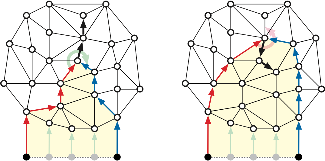
Call any directed edge \(u \mathord\to v\) properly shared by \(T_i\) and \(T_k\) if it satisfies the following recursive conditions:

• \(\mathit{pred}_i(v) = \mathit{pred}_k(v) = u\); in other words, \(u \mathord\to v\) is an edge in both \(T_i\) and \(T_k\).
• If \(\mathit{pred}_i(u) = \mathit{pred}_k(u)\), then the edge \(\mathit{pred}_i(u)\mathord\to u\) is properly shared.
• Otherwise, vertices \(\mathit{pred}_i(u)\), \(v\), \(\mathit{pred}_k(u)\) are ordered clockwise around \(u\).

We say that a properly shared edge \(u \mathord\to v\) is exposed if \(\mathit{pred}_i(u) \ne \mathit{pred}_k(u)\). For example, in Figure 2, both heavy black edges on the left are properly shared, but only the lower edge is exposed; the heavy black edges on the right are not properly shared.

Lemma: If \(u\mathord\to v\) is properly shared by \(T_i\) and \(T_k\), then \(\mathit{pred}_j(v) = u\) for all \(i\le j\le k\).

Proof:

First suppose \(u\mathord\to v\) is properly shared and exposed. Let \(\gamma\) be a simple closed curve obtained by concatenating \(\mathit{path}_k(u)\), the reversal of \(\mathit{path}_i(u)\), and a simple path from \(s_i\) to \(s_k\) through the outer face. (The shaded yellow region Figure 2 is the interior of \(\gamma\).) Each source vertex \(s_j\) is inside \(\gamma\), and \(v\) is outside \(\gamma\). So the Jordan curve theorem implies that \(\mathit{path}_j(v)\) must cross \(\gamma\). Uniqueness of shortest paths implies that \(\mathit{path}_j(v)\) cannot cross either \(\mathit{path}_i(v)\) or \(\mathit{path}_k(v)\). It follows that \(\mathit{path}_j(v)\) must contain \(u\), and thus \(\mathit{pred}_j(v) = u\).

Now suppose \(u\mathord\to v\) is properly shared but not exposed. Let \(p\) be the first vertex on \(\mathit{path}_i(v)\) that is also in \(\mathit{path}_k(v)\), and let \(p\mathord\to q\) be the first edge on the shortest path from \(p\) to \(v\) in \(H\). Our recursive definitions imply that \(p\mathord\to q\) is properly shared and exposed, so by the previous paragraph, for any index \(j\), we have \(\mathit{pred}_j(q) = p\) for all \(i\le j\le k\). It follows that \(T_j\) contains the entire shortest path from \(p\) to \(v\), and in particular, the edge \(u\mathord\to v\). \(\qquad\square\)

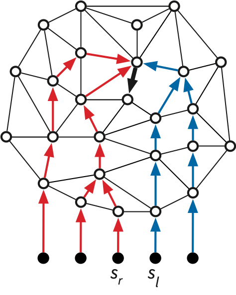
The converse of the previous lemma is not necessarily true; it is possible for \(\mathit{pred}_j(v) = u\) for every index \(j\) even though \(u\mathord\to v\) is not properly shared. Consider the reversed shortest path tree \(\overline{T}_v\) rooted at \(v\). Let \(s_l\) and \(s_r\) be the leftmost and rightmost source vertices in the subtree of \(\overline{T}_v\) rooted at \(u\). If this subtree contains every source vertex \(s_j\), then \(l = r+1 \bmod h\); intuitively, the subtree wraps around \(u\mathord\to v\) and meets itself at the boundary. See Figure 4 for an example. Edges of this form are not detected by the filtering algorithm.

Let \(m\) denote the number of vertices in \(H\). We can identify all properly shared edges in \(H\) in \(O(m)\) time using a preorder traversal of either \(T_i\) or \(T_k\). In particular, we can find all exposed edges leaving vertex \(u\) in \(\deg(u)\) time by visiting the darts into \(u\) in clockwise order—following the successor permutation—from \(\mathit{pred}_i(u)\mathord\to u\) to \(\mathit{pred}_k(u)\mathord\to u\).

Contraction

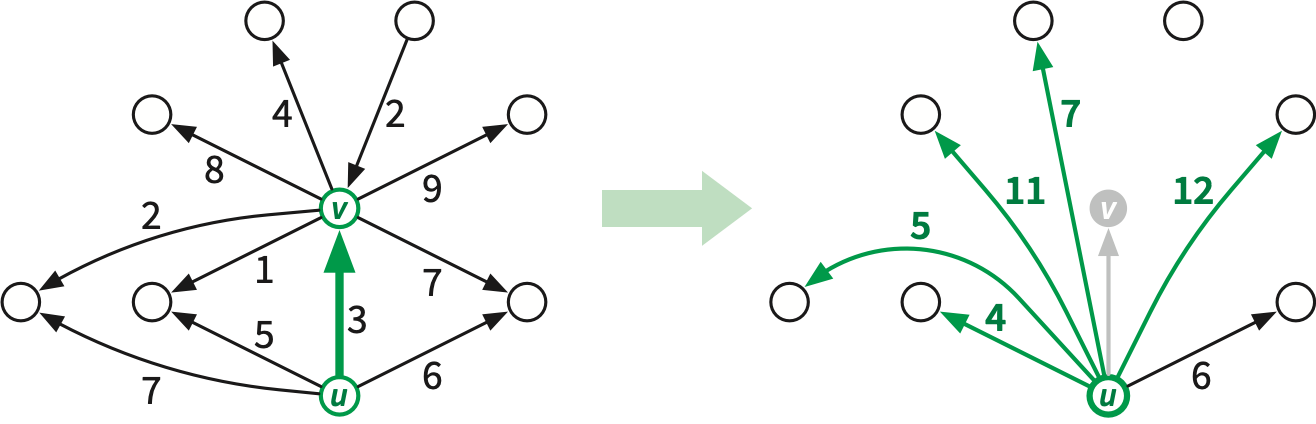
The main work of the filtering algorithm is contracting properly shared edges so that they need not be passed to recursive subproblems. Intuitively, we contract the edge \(u\mathord\to v\) into its tail \(u\), changing the tail of each directed edge \(v\mathord\to w\) from \(v\) to \(u\). Here are the steps in detail:

• Set \(\mathit{rep}(v) \gets u\)
• Set \(\mathit{off}(v) \gets \ell(u\mathord\to v)\)
• For every edge \(w\mathord\to v\):
  • Set \(\ell(w\mathord\to v) \gets \infty\)
• For every edge \(v\mathord\to w\):
  • Set \(\ell(v\mathord\to w) \gets \mathit{off}(v) + \ell(v\mathord\to w)\)
  • If \(\mathit{pred}_i(w)=v\), set \(\mathit{pred}_i(w)\gets u\)
  • If \(\mathit{pred}_k(w)=v\), set \(\mathit{pred}_k(w)\gets u\)
• Contract \(uv\) to \(u\)

The actual edge-contraction (in the second-to-last step) merges the successor permutations of \(u\) and \(v\) in \(O(1)\) time, as described in Lecture 10.

If \(u\) and \(v\) have any common neighbors, contracting \(v\) into \(u\) creates parallel edges, which we must resolve before passing the contracted map to \(\textsf{MSSP-prep}\). After all properly shared edges are contracted, we perform a global cleanup that identifies and resolves all families of parallel edges. Specifically, for each pair of neighboring vertices \(u\) and \(v\) in the contracted map, we choose on edge \(e\) between \(u\) and \(v\), change the dart weights of \(e\) to match the lightest darts \(u\mathord\to v\) and \(v\mathord\to u\), and then delete all other edges between \(u\) and \(v\). If we use hashing to recognize and collect parallel edges, the entire cleanup phase takes linear time.⁵

Contracting \(u\mathord\to v\) preserves the shortest-path distance from every source \(s_j\) to every other vertex (except the contracted vertex \(v\)). Moreover, for every source vertex \(s_j\) and every vertex \(w\) in the original map \(H\) including \(v\), contraction also maintains the following invariant, which allows us to recover shortest-path distances during the query algorithm. Let \(\mathit{dist}_j(w)\) denote the shortest-path distance from \(s_j\) to \(w\) in the original map \(H\), and let \(\mathit{dist}’_j(w)\) denote the corresponding distance in the current contracted map.

Key Invariant: For every vertex \(w\) of \(H\) and for every index \(j\) such that \(i\le j\le k\), we have \(\mathit{dist}_j(w) = \mathit{dist}’_j(\mathit{rep}(w)) + \mathit{off}(w)\).

When \(\textsf{Filter}\) begins, we have \(\mathit{dist}_j(w) = \mathit{dist}’_j(w)\) and \(\mathit{rep}(w) = w\) and \(\mathit{off}(w)=0\), so the Key Invariant holds trivially.

We contract properly shared edges in the same order they were discovered, following a preorder traversal of \(T_i\). This contraction order conveniently guarantees that we only contract exposed edges; contracting one exposed edge \(u \mathord\to v\) transforms each properly shared edge leaving \(v\) into an exposed properly shared edge leaving \(u\). This contraction order also guarantees that after contracting \(u\mathord\to v\), no edge into \(u\) will ever be contracted. It follows that we change the tail of each edge (and therefore the predecessors of each vertex) at most once, and the Key Invariant is maintained. We conclude:

Lemma: \(\textsf{Filter}(H, i, k)\) identifies and contracts all properly shared edges in \(H\) in \(O(S(m) + m)\) time, where \(m = |V(H)|\). Moreover, after \(\textsf{Filter}(H, i, k)\) ends, the Key Invariant holds.

Distance Queries

Each call to \(\textsf{Filter}(H,i,k)\) creates a record storing the following information:

• indices \(i\) and \(k\)
• for each vertex \(v\) of the input map \(H\):⁶
  • shortest-path distances \(\mathit{dist}_i(v)\) and \(\mathit{dist}_k(v)\)
  • the representative vertex \(\mathit{rep}(v)\)
  • the offset \(\mathit{off}(v)\).

The recursive calls to \(\textsf{MSSP-Prep}\) assemble these records into a binary tree, mirroring the tree of recursive calls, connected by \(\mathit{left}\) and \(\mathit{right}\) pointers.

The query algorithm \(\textsf{MSSP-query}(\mathit{Rec},j,v)\) takes as input a recursive-call record \(\mathit{Rec}\), a source index \(j\), and a vertex \(v\), satisfying two conditions:

• \(\mathit{Rec}.i \le j\le \mathit{Rec}.k\)
• \(v\) is a vertex of the input map \(H\) to the recursive call to \(\textsf{MSSP-Prep}\) that created \(\mathit{Rec}\).

The output of \(\textsf{MSSP-query}(\mathit{Rec},j,v)\) is the shortest-path distance from \(s_j\) to \(v\) in \(\Sigma\). The query algorithm follows straightforwardly from the Key Invariant:

• if \(j=i\), return \(\mathit{Rec}.\mathit{dist}_i[v]\)
• else if \(j=k\), return \(\mathit{Rec}.\mathit{dist}_k[v]\)
• else if \(j \le \mathit{Rec}.\mathit{left}.k\), return \(\textsf{MSSP-query}(\mathit{Rec}.\mathit{left}, j, \mathit{Rec}.\mathit{rep}[v]) + \mathit{Rec}.\mathit{off}[v]\)
• else return \(\textsf{MSSP-query}(\mathit{Rec}.\mathit{righ}, j, \mathit{Rec}.\mathit{rep}[v]) + \mathit{Rec}\mathord.\mathit{off}[v]\)

Because the recursion tree has depth \(O(\log h)\), the query algorithm runs in \(O(\log h)\) time.

Space and Time Analysis

It remains only to bound the size of our data structure and the running time of \(\textsf{MSSP-Prep}\). The key claim is that the total size of all input maps at any level of the recursion tree is \(O(n)\).

Contraction sharing lemma: Contracting one properly shared edge neither creates nor destroys other properly shared edges.

Proof:

Fix a map \(H\) and source indices \(i\) and \(k\). Let \(u\mathord\to v\) be an edge in \(H\) that is properly shared by \(T_i\) and \(T_k\). Let \(H’ = H / u{\to}v\), with dart weights adjusted as described above, and let \(T’_i\) and \(T’_k\) denote the shortest path trees rooted at \(s_i\) and \(s_k\) in \(H’\).

First, because contraction preserves shortest paths, we can easily verify that \(T’_i = T_i / u{\to}v\) and \(T’_k = T_k / u{\to}v\). It follows that an edge in \(H\) is shared by \(T_i\) and \(T_k\) if and only if the corresponding edge in \(H’\) is shared by \(T’_i\) and \(T’_k\).

Now consider any edge \(x{\to}y \in T_i \cap T_k\) that is not \(u{\to}v\). We must have \(y\ne v\), because each vertex has only one predecessor in any shortest-path tree. Let \(w\) be the first node on the shortest path from \(s_i\) to \(x\) in \(H\) that is also on the shortest path from \(s_k\) to \(x\), so the entire shortest path from \(w\) to \(y\) is shared by \(T_i\) and \(T_k\). Consider three paths:

• \(\alpha =\) the shortest path from \(s_i\) to \(w\)

• \(\beta =\) the reverse of the shortest path from \(w\) to \(y\)

• \(\gamma =\) the shortest path from \(s_k\) to \(w\)

Then \(x{\to}y\) is properly shared if and only if (the last edges of) \(\alpha\), \(\beta\), and \(\gamma\) are incident to \(w\) in clockwise order. The definition of properly shared implies \(v=w\), so \(w\) is also a vertex in \(H’\). Contracting \(u{\to}v\) might shorten one of the three paths to \(w\), but it cannot change their cyclic order around \(w\). We conclude that \(x{\to}y\) is properly shared in \(H\) if and only if \(x{\to}y\) (or \(u{\to}y\) if \(x=v\)) is properly shared in \(H’\). \(\qquad\square\)

The contraction sharing lemma implies by induction that every call to \(\textsf{Filter}(H, i, k)\) outputs the same contracted map as \(\textsf{Filter}(\Sigma, i, k)\). In particular, an edge \(u\mathord\to v\) in \(H\) is properly shared by two shortest-oath trees in \(H\) if and only if the corresponding edge in \(\Sigma\) (which may have a different tail vertex) is properly shared by the corresponding trees in \(\Sigma\). So from now on, “properly shared” always implies “in the top level map \(\Sigma\)”.

Corollary: For all indices \(i\le i’<k’\le k\), if \(u{\to}v\) is properly shared by \(T_i\) and \(T_k\), then \(u{\to}v\) is properly shared by \(T_{i’}\) and \(T_{k’}\).

Corollary: The vertices of \(\textsf{Filter}(\Sigma, i, k)\) are precisely the vertices \(v\) such that no edge into \(v\) is properly shared by \(T_i\) and \(T_k\).

Fix any vertex \(v\) of \(\Sigma\). We call an index \(j\) interesting if \(\mathit{pred}_j(v)\mathord\to v\) is not properly shared by \(T_j\) and \(T_{j+1}\).

Lemma: Every vertex \(v\) of \(\Sigma\) has at most \(\deg(v)\) indices.

Proof:

Equivalently, \(j\) is interesting to \(v\) if either of the following conditions holds:

• \(\mathit{pred}_j(v) \ne \mathit{pred}_{j+1}(v)\).

• \(\mathit{pred}_0(v) = \mathit{pred}_1(v) = \cdots = \mathit{pred}_{h-1}(v) = u\) and the paths \(\mathit{path}_j(u)\) and \(\mathit{path}_{j+1}(u)\) “wrap around” \(u \mathord\to v\).

The Disk-Tree Lemma implies that the first condition holds for at most \(\deg(v)\) indices \(j\). If the first condition never holds (that is, if \(\mathit{pred}_j(v)\) is the same for index \(j\)), then the second condition holds for exactly one index \(j\); otherwise the second condition never holds. \(\qquad\square\)

Lemma: Each vertex \(v\) appears in at most \(2\deg(v)\) subproblems at each level of the recursion tree.

Proof:

The children \(\mathit{Rec}.\mathit{left}\) and \(\mathit{Rec}.\mathit{right}\) of any recursion record \(\mathit{Rec}\) store information about \(v\) and if and only if at least one index \(j\) such that \(\mathit{Rec}.i\le j\le \mathit{Rec}.k\) is interesting to \(v\). \(\qquad\square\)

Theorem: \(\textsf{MSSP-Prep}(\Sigma, 0, h-1)\) builds a data structure of size \(O(n\log h)\) in \(O(S(n)\log h)\) time.

Proof:

The total number of vertices in all subproblems at the same level of the recursion tree is at most \(\sum_v 2\deg(v) \le 4\cdot|E(\Sigma)| \le 4(3n-6) = 12n-24\) by Euler’s formula, since \(\Sigma\) is a simple planar map. Each recursion record uses \(O(1)\) space per vertex, so the total space used at any level is \(O(n)\). Similarly, the time spent in any subproblem is at most \(O(S(n)/n)\) per vertex, so the total time spent in each level of the recursion tree is \(O(S(n))\).

Finally, the recursion tree has \(O(\log h)\) levels. \(\qquad\square\)

References

1. Debarati Das, Evangelos Kipouridis, Maximilian Probst Gutenberg, and Christian Wulff-Nilsen. A simple algorithm for multiple-source shortest paths in planar digraphs. Proc. 5th Symp. Simplicity in Algorithms, 1–11, 2022.

2. David Eisenstat. Toward Practical Planar Graph Algorithms. Ph.D. thesis, Comput. Sci. Dept., Brown Univ., May 2014.

3. Jacob Holm, Giuseppe F. Italiano, Adam Karczmarz, Jakub Łącki, Eva Rotenberg, and Piotr Sankowski. Contracting a planar graph efficiently. Proc. 25th Ann. Europ. Symp. Algorithms, 50:1–50:15, 2017. Leibniz Int. Proc. Informatics 87, Schloss Dagstuhl–Leibniz-Zentrum für Informatik. arXiv:1706.10228.

4. Frank Kammer and Johannes Meintrup. Succinct planar encoding with minor operations. Preprint, January 2023. arXiv:2301.10564.

5. Robert E. Tarjan and Renato F. Werneck. Dynamic trees in practice. J. Exper. Algorithmics 14:5:1–5:21, 2009.

6. Renato Werneck. Design and Analysis of Data Structures for Dynamic Trees. Ph.D. thesis, Dept. Comput. Sci., Princeton Univ., April 2006. Tech. Rep. TR-750-06.