Let \(\Sigma\) be an arbitrary planar map, with non-negative weights on its vertices, edges, and/or faces that sum to \(W\). A simple cycle \(C\) in a planar map \(\Sigma\) is a balanced cycle separator if the total weight of all vertices, edges, and faces on either side of \(C\) is at most \(3W/4\). As long as each vertex, edge, or face of \(\Sigma\) has weight at most \(W/4\), there is a balanced cycle separator with at most \(O(\sqrt{n})\) vertices; moreover, we can compute such a cycle in \(O(n)\) time.
Before we consider separators in planar graphs, let’s consider the simpler case of trees. Here a balanced separator is a single edge that splits the tree into two subtrees of roughly equal weight. Tree separators were first studied by Camille Jordan
Let \(T = (V, E)\) be an unrooted tree in which every vertex has degree at most \(3\). Intuitively, \(T\) is a “binary” tree, but without a root and without a distinction between left and right children. (This bounded-degree assumption is necessary.) Assign each vertex \(v\) a non-negative weight \(w(v)\) and let \(W := \sum_v w(v)\).
For any vertex \(v\), let \(W(v)\) denote the total weight of \(v\) and its descendants; for example, \(W(r) = W\). For any non-leaf vertex \(v\), label its children \(\textsf{heft}(v)\) and \(\textsf{lite}(v)\) so that \(W(\textsf{heft}(v)) \ge W(\textsf{lite}(v))\) (breaking ties arbitrarily).
Starting at the root \(r\), follow pointers down to the first vertex \(x\) such that \(W(\textsf{heft}(x)) \le W/4\). Then we immediately have \[ \begin{aligned} W/4 &< W(x) \\ &= W(\textsf{heft}(x)) + W(\textsf{lite}(x)) + w(x) \\ &\le 2\cdot W(\textsf{heft}(x)) + w(x) \\ &\le 3W/4. \end{aligned} \] Let \(e\) be the edge between \(x\) and its parent. The two components of \(T\setminus e\) have total weight \(W(x) \le 3W-4\) and \(W - W(x) < 3W/4\). \(\qquad\square\).
It’s easy to see that the upper bounds on vertex degree and vertex weight are both necessary. This separator lemma has several variants; I’ll mention just a few without proof:
Now let \(\Sigma\) be a planar triangulation. Assign each face \(f\) a non-negative weight \(w(f) \le W/4\), where \(W := \sum_f w(f)\). (Again, the upper bounds on face degree and face weight are both necessary.) A cycle \(C\) in \(\Sigma\) is a balanced separator if the total weight on either side of \(C\) is at most \(3W/4\).
Let \(T\) be an arbitrary spanning tree of \(\Sigma\). For any non-tree edge \(e\), the fundamental cycle \(\textsf{cycle}(T, e)\) is the unique cycle in \(T+e\), consisting of \(e\) and the unique path in \(T\) between the endpoints of \(e\).
We can extend this lemma to the setting where vertices and edges also have weights, in addition to faces. Let \(w\colon V\cup E\cup F \to \mathbb{R}_+\) be the given weight function. Define a new face-weight function \(w’\colon F\to\mathbb{R}_+\) by moving the weight of each vertex and edge to some incident face.
Unfortunately, fundamental cycles can be quite long. For any particular map \(\Sigma\), we can minimize the maximum length of all fundamental cycles using a breadth-first search tree from the correct root vertex as our spanning tree \(T\), but in the worst case, every balanced fundamental cycle separator has length \(\Omega(n)\).
For most applications of balanced separators, breadth-first fundamental cycles are usually the best choice in practice; see the detailed experimental analysis by Fox-Epstein et al. [1].
A second easy method for computing separators is to consider the levels of a breadth-first search tree. For the moment, let’s assume that the vertices of \(\Sigma\) are weighted. For each integer \(\ell\), let \(V_\ell\) denote the vertices \(\ell\) steps away from the root vertex of \(T\). By computing a weighted median, we can find a level \(V_m\) such that the total vertex weight in any component of \(\Sigma\setminus V_m\) is at most \(W/2\).
There are two obvious problems with this separator construction. The less serious problem is that the medial level \(V_m\) is not a cycle; it’s just a cloud of vertices. Many applications of planar separators don’t actually require cycle separators, but most of the applications we’ll see in this class do. The more serious problem is size; in the worst case, the set \(V_m\) could contain a constant fraction of the vertices.
When Richard Lipton and Robert Tarjan introduced planar separators in 1979, they did not consider cycle separators. Rather, they proved that there is always a subset \(S\) of \(O(\sqrt{n})\) vertices such that any component of \(\Sigma\setminus S\) has at most \(2n/3\) vertices. Lipton and Tarjan’s construction combines fundamental cycle separators and BFS-level separators. I will not describe their construction in detail, partly because we really do need cycles, and partly because most of their ideas show up in the next section.
Gary Miller was the first to prove that small balanced cycle separators exist, in 1986. The following refinement of Miller’s algorithm is based on later proofs by Philip Klein, Shay Mozes, and Christian Sommer (2013) and Sariel Har-Peled and Amir Nayyeri (2018). Miller’s key idea was to generalize our notion of “level” from vertices to faces.1
As in our earlier setup, Let \(\Sigma\) be a simple planar triangulation with weighted faces, where no individual face weight is too large. Let \(T_0\) be a breadth-first search tree, and suppose the fundamental cycle \(\textsf{cycle}(T_0, xy)\) is a balanced separator. If this cycle has length \(O(\sqrt{n})\), we are done, so assume otherwise.
Let \(r\) denote the least common ancestor of \(x\) and \(y\), and let \(T\) be a breadth-first search tree rooted at \(r\). The cycle \(\textsf{cycle}(T, xy) = \textsf{cycle}(T_0, xy)\) is still a balanced separator.
For any vertex \(v\), let \(\textsf{level}(v)\) denote the breadth-first distance from \(r\) to \(v\). Without loss of generality, assume \(\textsf{level}(x) \le \textsf{level}(y)\). Then for any face \(f\), let \(\textsf{level}(f)\) denote the maximum level among the three vertices of \(f\). A face at level \(\ell\) has vertices only at levels \(\ell\) and \(\ell-1\). Let \(o\) denote the outer face of \(\Sigma\), and without loss of generality, assume that \(L = \textsf{level}(o) = \max_f \textsf{level}(f)\).
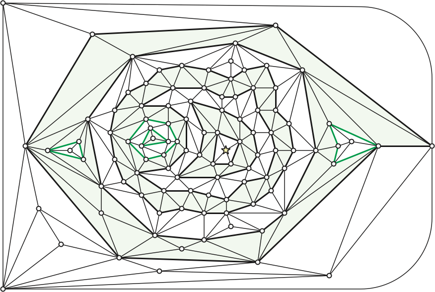
For any integer \(\ell\), let \(U_{\le\ell}\) denote the union of all faces with level at most \(\ell\), and let \(C_\ell\) be the outer boundary of \(U_{\le\ell}\). Trivially \(U_{\le 0} = \varnothing\) and therefore \(C_0 = \varnothing\). Similarly, fr any \(\ell\ge L\), we have \(U_{\le \ell} = \mathbb{R}^2\) and therefore \(C_\ell = \varnothing\).
By construction \(C_\ell\) consists of one or more simple cycles, any two of which share at most one vertex. Let \(C\) be the simple cycle in \(C_\ell\) that contains \(r\) in its interior. and let \(v\) be any vertex of \(C_\ell\setminus C\). Let \(u\) be the second-to-last vertex on the shortest path from \(r\) to \(v\). Vertex \(u\) has level \(\ell-1\) and therefore does not lie on \(C\); moreover, because \(v\not\in C\), vertex \(u\) cannot lie in the interior of \(C\). The Jordan curve theorem implies that the shortest path from \(u\) to \(r\) crosses \(C\), but this is impossible, because levels decrease monotonically along that path. We conclude that \(C_\ell = C\), proving part (b).
Part (c) follows immediately from part (a).
Finally, the vertices of \(\textsf{cycle}(T, xy)\) lie on two shortest paths from \(r\), one to \(x\) and the other to \(y\). Levels increase monotonically along any shortest path from \(r\). Thus, by part (a), the shortest paths from \(r\) to \(x\) and \(y\) each share at most one vertex with \(C_\ell\). \(\qquad\square\)
Let \(m\) be the largest integer such that the total weight of all faces inside \(C_m\) is at most \(W/2\). Then the total weight of the faces outside \(C_{m+1}\) is also at most \(W/2\). If either of these cycles is a balanced cycle separator of length \(O(\sqrt{n})\), we are done, so assume otherwise. We choose two level cycles \(C^-\) and \(C^+\) as follows.2
Consider the set of cycles \(\mathcal{C}^- = \{C_\ell \mid m-\sqrt{n} < \ell \le m\}\). These \(\sqrt{n}\) cycles contain at most \(n\) vertices, and therefore some cycle \(C^-\) in this set must have length less than \(\sqrt{n}\). By construction, the total weight of all faces inside \(C^-\) is at most \(W/2\).
Similarly, consider the set \(\mathcal{C}^+ = \{C_\ell \mid m < \ell \le m + \sqrt{n}\}\). These \(\sqrt{n}\) cycles contain at most \(n\) vertices, and therefore some cycle \(C^+\) in this set must have length less than \(\sqrt{n}\). By construction, the total weight of all faces outside \(C^+\) is at most \(W/2\).
Let \(\pi_x\) denote the portion of the shortest path from \(r\) to \(x\) with levels between \(a\) and \(b\), and define \(\pi_y\) similarly. By construction, each of these paths has length at most \(2\sqrt{n}\). Let \(\Theta\) denote the graph \(C^- \cup C^+ \cup \pi_x \cup \pi_y\), as shown in the figure below. This subgraph of \(\Theta\) has at most \(4\sqrt{n}\) vertices and edges. We label the four faces of \(\Theta\) as follows:
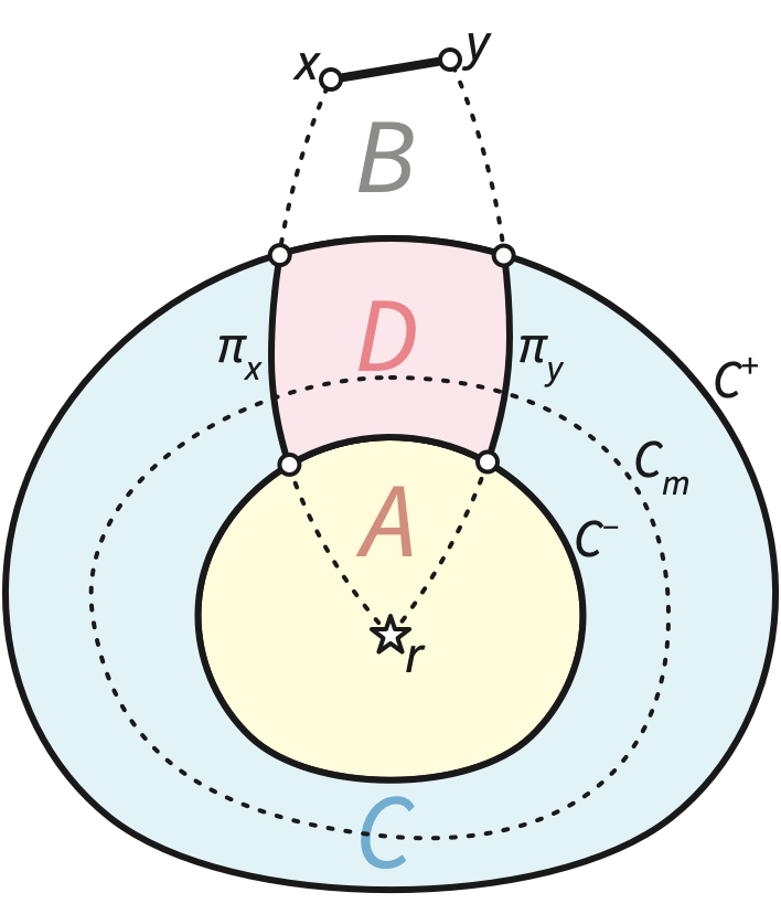
Let \(W(S)\) denote the total weight of the set of faces \(S\). By construction we have \[ \begin{aligned} W(A) & \le W/2, &&& W(B) & \le W/2, &&& W(C) & \le 3W/4, &&& W(D) & \le 3W/4. \end{aligned} \] At least one of these four regions contains total weight at least \(W/4\); the boundary of that region is a balanced cycle separator of length \(O(\sqrt{n})\).
Most divide-and-conquer algorithms that use cycle separators do not delete the separator vertices to obtain smaller subgraphs. Rather, the algorithms slice the planar map along the cycle separator to obtain smaller maps, called pieces of the original map, one containing the faces inside the cycle and the other containing the faces outside. Both pieces contain a copy of the \(O(\sqrt{n})\) vertices and edges of the separator. Thus, the total size of all subproblems is larger at deeper levels of the recursion tree, but because that increase is sublinear, we can ignore it when solving the resulting divide-and-conquer recurrences.
An \(r\)-division is a decomposition of a planar map into \(n/r\) pieces, each of which has \(O(r)\) vertices and \(O(\sqrt{r})\) boundary vertices (shared with other pieces). An \(r\)-division is good if each piece is a disk with \(O(1)\) holes. For any \(r\), we can construct a good \(r\)-division by recursively slicing the input triangulation along balanced cycle separators. In fact, this subdivision strategy computes a subdivision hierarchy that includes good \(r\)-divisions for arbitrary values of \(r\).
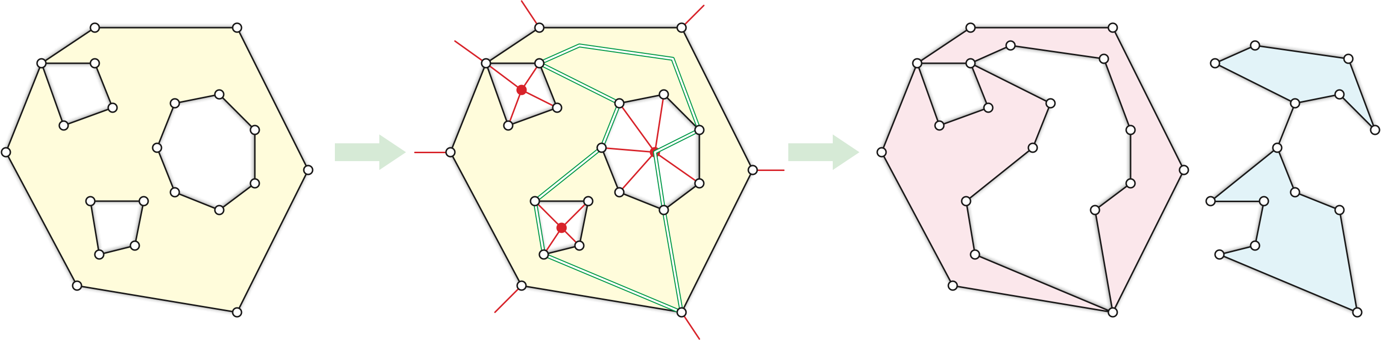
In each recursive call, we are given a region \(R\), which is a connected subcomplex of the original triangulation \(\Sigma\). Any face of the region \(R\) that is not a face of \(\Sigma\) is called a hole; any vertex of \(R\) that is incident to a hole is a boundary vertex of \(R\). To split \(R\) into two smaller regions, we first triangulate \(R\) by inserting an artificial vertex \(v_h\) inside each hole \(h\), along with artificial edges connecting \(v_h\) to each corner of \(h\). We then compute a cycle separator in the resulting triangulation \(R’\), splitting it into two smaller triangulated regions \(R’_0\) and \(R’_1\). Finally, we delete the artificial vertices and edges from \(R’_0\) and \(R’_1\) to get the final regions \(R_0\) and \(R_1\).
To simultaneously bound the number of vertices, the number of boundary vertices, and the number of holes in the final regions, we cycle through three different vertex weights at different levels of recursion. Specifically, at recursion depth \(l\), we weight the vertices as follows:
Let \(T_r(n, b, h)\) denote the time to compute a good \(r\)-division for a region with \(n\) vertices, \(b\) boundary vertices, and \(h\) holes. Expanding out three levels of recursion, we have \[ T_r(n, b, h) = O(n + h) + \sum_{i=1}^8 T_r(n_i, b_i, h_i), \] where \[ \begin{aligned} \sum_{i=1}^8 n_i &\le n + O(\sqrt{n}) & \sum_{i=1}^8 b_i &\le b + O(\sqrt{n}) & \sum_{i=1}^8 h_i &\le h + O(1) \\ \max_i n_i &\le 3n/4 + O(\sqrt{n}) & \max_i b_i &\le 3b/4 + O(\sqrt{n}) & \max_i h_i &\le 3h/4 + O(1) \end{aligned} \] for suitable absolute big-Oh constants. The recursion stops when the number of vertices in each piece is \(O(r)\). Every leaf in the recursion tree has depth at most \(O(\log (n/r))\), and there are at most \(O(n/r)\) such leaves. One can prove by induction that in every recursive subproblem, the number of boundary vertices is at most \(O(\sqrt{r})\) and the number of holes is at most \(O(1)\), so we end with a good \(r\)-division. We perform \(O(n)\) work at every level of recursion, so the overall running time of the algorithm is \(T_r(n, 0, 0) = O(n \log(n/r))\). In particular, if \(r = O(1)\), the entire algorithm runs in \(O(n\log n)\) time.
Theorem: Given a planar triangulation \(\Sigma\) with \(n\) vertices, we can compute a recursive subdivision of \(\Sigma\), containing good \(r\)-divisions of \(\Sigma\) for every \(r \ge r_0\), in \(O(n \log (n/r_0))\) time.
Corollary: Given a planar triangulation \(\Sigma\) with \(n\) vertices and an integer \(r\), we can compute a good \(r\)-division of \(\Sigma\) in \(O(n \log (n/r))\) time.
Some applications of separators actually require a nested sequence of good \(r\)-divisions with exponentially decreasing values of \(r\). For any vector \(\vec{r} = (r_1, r_2, \dots, r_t)\) where \(r_i < r_{i-1}/\alpha\) for some suitable constant \(\alpha\), a good \(\vec{r}\)-division of a planar map \(\Sigma\) consists of a good \(r_1\)-division \(\mathcal{R}_1\) of \(\Sigma\) and (unless \(t=1\)) a good \((r_2, \dots, r_t)\)-division of each piece of \(\mathcal{R}_1\). We can easily extract a good \(\vec{r}\)-division from any good subdivision hierarchy in \(O(n)\) time.
Corollary: Given a planar triangulation \(\Sigma\) with \(n\) vertices, and any exponentially decreasing vector \(\vec{r} = (r_1, r_2, \dots, r_t)\), we can construct a good \(\vec{r}\)-division of \(\Sigma\) in \(O(n \log (n/r_t))\) time.
Greg Frederickson introduced \(r\)-divisions (based on non-cycle separators) in 1989. The current definition of good \(r\)-division was proposed by Philip Klein and Sairam Subramanian in 1998. The three-phase algorithm I’ve just described was first proposed by Jittat Fakcharoenphol and Satish Rao in 2006, and extended to \(\vec{r}\)-divisions by Philip Klein, Shay Mozes, and Christian Sommer in 2013.
This is not the fastest algorithm known for computing good \(r\)-divisions. A different algorithm for constructing a good \(r\)-division in \(O(n\log r + O(n/\sqrt{r})\log n)\) time was described by Giuseppe Italiano, Yahav Nussbaum, Piotr Sankowski, and Christian Wulff-Nilsen in 2011.
In 1996, Lyudmil Aleksandrov and Hristo Djidjev described an \(O(n)\)-time algorithm to construct \(r\)-divisions based on Lipton-Tarjan separators, for any given \(r\). In 2013, Lars Arge, Freek van Walderveen, and Norbert Zeh described an algorithm to construct a single good \(r\)-division in \(O(n)\) time. [[[How do these algorithms work?]]]
The first linear-time algorithm for building a subdivision hierarchy containing \(r\)-divisions for every \(r\) was described by Michael Goodrich in 1996. Klein, Mozes, and Sommer described a similar algorithm to compute a good subdivision hierarchy in \(O(n)\) time.3 Both of these algorithms use dynamic forest data structures (to maintain tree-cotree decompositions of the pieces, identify fundamental cycle separators, compute least common ancestors, and compute the weight enclosed by short cycles), along with several other data structures.
In the next lecture we’ll see how to use good \(r\)-divisions to compute shortest paths quickly.
Lyudmil Aleksandrov and Hristo Djidjev. Linear algorithms for partitioning embedded graphs of bounded genus. SIAM J. Discrete Math. 9(1):129–150, 1996.
Lars Arge, Freek van Walderveen, and Norbert Zeh. Multiway simple cycle separators and {I/O}-efficient algorithms for planar graphs. Proc. 24th Ann. ACM-SIAM Symp. Discrete Algorithms, 901–918, 2013.
Jittat Fakcharoenphol and Satish Rao. Planar graphs, negative weight edges, shortest paths, and near linear time. J. Comput. Syst. Sci. 72(5):868–889, 2006.
Eli Fox-Epstein, Shay Mozes, Phitchaya Mangpo Phothilimthana, and Christian Sommer. Short and simple cycle separators in planar graphs. ACM J. Exp. Algorithmics 21(1):2.2:1–2.2:24, 2016.
Greg N. Frederickson. Fast algorithms for shortest paths in planar graphs with applications. SIAM J. Comput. 16(8):1004–1004, 1987.
Michael T. Goodrich. Planar separators and parallel polygon triangulation. J. Comput. Syst. Sci. 51(3):374–389, 1995.
Sariel Har-Peled and Amir Nayyeri. A simple algorithm for computing a cycle separator. Preprint, September 2017. arXiv:1709.08122.
Giuseppe F. Italiano, Yahav Nussbaum, Piotr Sankowski, and Christian Wulff-Nilsen. Improved algorithms for min cut and max flow in undirected planar graphs. Proc. 43rd Ann. ACM Symp. Theory Comput., 313–322, 2011.
Camille Jordan. Sur les assemblages de lignes. J. Reine Angew. Math. 70:185–190, 1869.
Philip N. Klein, Shay Mozes, and Christian Sommer. Structured recursive separator decompositions for planar graphs in linear time. Proc. 45th Ann. ACM Symp. Theory Comput., 505–514, 2013. arXiv:1208.2223.
Philip N. Klein and Sairam Subramanian. A fully dynamic approximation scheme for shortest paths in planar graphs. Algorithmica 22(3):235–249, 1998.
Richard J. Lipton and Robert E. Tarjan. A separator theorem for planar graphs. SIAM J. Applied Math. 36(2):177–189, 1979.
Richard J. Lipton and Robert Endre Tarjan. Applications of a planar separator theorem. SIAM J. Comput. 9:615–627, 1980.
Gary L. Miller. Finding small simple cycle separators for 2-connected planar graphs. J. Comput. System Sci. 32(3):265–279, 1986.
Fox-Eppstein et al. [1] describe an arguably simpler algorithm that uses a dual breadth-first search tree rooted at the outer face to define face levels, instead of a primal breadth-first search tree.↩︎
I am ignoring two extreme cases. First, if \(m < \sqrt{n}\), we define \(C^- = \varnothing\); similarly, if \(m > \textsf{level}(y) - \sqrt{n}\), we define \(C^+ = \varnothing\). Handling these special cases in the rest of the construction is straightforward.↩︎
The two 1996 results are completely independent; so are the two 2013 results.↩︎