One of the most important applications of separators and \(r\)-divisions in planar graphs is faster algorithms to computer shortest paths. Most of these faster algorithms rely on an implicit representation of shortest-path distances called the dense distance graph, first explicitly described by Jittat Fakcharoenphol and Satish Rao in 2001, but already implicit in Lipton, Rose, and Tarjan’s 1979 nested dissection algorithm, which we will discuss shortly.
Let \(\Sigma\) be a simple planar map with weighted darts; for now we’ll assume that all edge weights are non-negative. If necessary, add infinite-weight edges so that \(\Sigma\) is a simple triangulation. Recall that a good \(r\)-division of \(\Sigma\) is a subdivision of \(\Sigma\) into \(O(n/r)\) pieces \(R_1, R_2, \dots\) satisfying three conditions:
Fix a good \(r\)-division \(\mathcal{R}\). For each piece \(R_i \in \mathcal{R}\), let \(X_i\) be a complete directed graph over the boundary vertices of \(R_i\), where each dart \(u{\to} v\) is weighted by the shortest-path distance in \(R_i\) from its tail \(u\) to its head \(v\). The dense distance graph is the union of these \(O(n/r)\) weighted cliques. Altogether, the dense distance graph has \(n’ = O(n/\sqrt{r})\) vertices—only the boundary vertices of the pieces of the \(r\)-division—and \(m’ = O(n)\) weighted darts.
Assuming all dart weights are non-negative, we can compute all \(O(r)\) boundary-to-boundary shortest-path distances in each piece \(R_i\) in \(O(r\log r)\) time, by running the multiple-source shortest-path algorithm once for each hole in \(R_i\), using Dijkstra’s algorithm to compute the initial shortest-path tree. Thus, the overall time to compute the dense-distance graph is \(O(n\log r)\).
Next we compute the shortest-path distance from \(s\) to every boundary vertex of the \(r\)-division by running Dijkstra’s algorithm in the dense distance graph. If we implement Dijkstra’s algorithm using Fibonacci heaps, this step takes \(O(n’\log n’ + m’) = O((n/\sqrt{r})\log n + n)\) time.
Finally, for each piece \(P\), we attach an artificial course \(s’\) to each boundary vertex \(u\) with an edge with length \(\textsf{dist}(s,u)\), and compute a shortest path tree in \(P\) from \(s’\) using Dijkstra’s algorithm. This step takes \(O(r\log r)\) time per piece, or \(O(n\log r)\) time overall.
The overall running time of our algorithm is \(O(n\log r + (n/\sqrt{r})\log n)\). In particular, if we set \(r = O(\log^2 n)\), the running time is \(O(n\log\log n)\). \(\qquad\square\)
Let me reiterate that this analysis assumes that we are using the parametric multiple-source shortest path algorithm to construct the dense-distance graph. If we try to use the more recent contraction-based MSSP algorithm of Das et al. instead, we end up with two mutually recursive algorithms, one computing single-course shortest paths, the other computing multiple-source shortest paths. The running time of the resulting single-source shortest-path algorithm is \(O(n\,\log\log n\, \log\log\log n\, \log\log\log\log n\cdots)\).
The idea to use \(r\)-divisions to speed up planar shortest paths is due to Greg Frederickson, who described an algorithm that runs in \(O(n\sqrt{\log n})\) time in 1987. Ten years later, Monika Henzinger, Philip Klein, Satish Rao, and Sairam Subramanian described an algorithm that runs in \(O(n)\) time. Both of these algorithms predate both good \(r\)-divisions and Klein’s multiple-source shortest-path algorithm. Instead, these algorithms are variants of Dijkstra’s algorithm that recursively relax pieces of a carefully chosen recursive separator decomposition, instead of relaxing individual edges. Unlike the \(O(n\log\log n)\) algorithm I’ve described above, which relies on good \(r\)-divisions and planarity, the \(O(n)\)-time algorithm of Henzinger et al. generalizes directly to any minor-closed family of graphs with bounded vertex degrees; the bounded-degree restriction was later removed by Tazari and Müller-Hannemann.
Depending on which textbook you read, Dijkstra’s algorithm is either no longer correct or no longer efficient when some darts of the input graph have negative weight. In particular, if \(\Sigma\) contains negative darts, we can no longer solve the multiple-source shortest-path problem in \(O(n\log n)\) time, because we don’t know how compute the initial shortest-path trees that quickly.1
The standard shortest-paths algorithm for graphs with negative edges is Bellman-Ford, which runs in \(O(mn)\) time; in particular, for simple planar graphs with \(n\) vertices, Bellman-Ford runs in \(O(n^2)\) time. But just as we beat Dijkstra’s algorithm, we can beat Bellman-Ford when the underlying graph is planar.
The following generalized nested dissection algorithm, proposed by Richard Lipton, Donald Rose, and Robert Tarjan in 1979, was one of the earliest applications of planar separators. (The original nested dissection algorithm, proposed by Alan George in 1973, applied only to square grid graphs.) Although their algorithm was originally designed for abstract planar graphs rather than planar maps, the presentation and analysis are simpler if we use good \(r\)-divisions, which require a planar embedding.
We are given a simple planar graph (sic) \(G\) with asymmetrically weighted darts, where some of the darts weights may be negative, and a source vertex \(s\). At a very high level, our strategy is to delete one vertex of \(G\) using a star-mesh transformation, compute shortest-path distances from \(s\) to every remaining vertex of \(G\), and finally compute the shortest-path distance from \(s\) to \(v\). A star-mesh transformation adds or reweights edges between the neighbors of the deleted vertex \(v\) to restore shortest-path distances. Specifically, if there is no edge \(uw\) between two neighbors \(u\) and \(w\), we add one with dart weights \[ \begin{aligned} \ell(u{\to}w) &\gets \ell(u{\to}v) + \ell(v{\to}w)\\ \ell(w{\to}u) &\gets \ell(w{\to}v) + \ell(v{\to}u); \end{aligned} \] on the other hand, if edge \(uw\) already exists, we change its dart weights as follows: \[ \begin{aligned} \ell(u{\to}w) &\gets \min \big\{ \ell(u{\to}w),~ \ell(u{\to}v) + \ell(v{\to}w) \big\} \\ \ell(w{\to}u) &\gets \min\big\{ \ell(w{\to}u),~ \ell(w{\to}v) + \ell(v{\to}u) \big\} \end{aligned} \] These changes preserve shortest-path distances from any vertex except \(v\) to any other vertex except \(v\).2 With the appropriate graph data structures, deleting \(v\) takes \(O(\deg(v)^2)\) time.
After the Recursion Fairy computes distances from \(s\) to all other vertices, we can recover the distance from \(s\) to \(v\) by brute force in \(O(\deg(v))\) time: \[ \textsf{dist}(v) \gets \min_{u{\to}v} \big\{\textsf{dist}(u) + \ell(u{\to}v)\big\} \] In both running times, \(\deg(v)\) refers to the degree of \(v\) when \(v\) is eliminated, not in the original graph \(G\). Different elimination orders can lead to different vertex degrees and therefore different running times. Star-mesh transformations do not preserve planarity, but this elimination process works for arbitrary graphs.
Lipton, Rose, and Tarjan recursively construct an elimination order for planar graphs as follows. Let \(S\) be a balanced separator that contains the source vertex \(s\), and let \(A\) and \(B\) be a partition of the vertices \(V\setminus S\) so that there is no edge directly from \(A\) to \(B\). We first recursively eliminate all vertices in \(A\), then recursively eliminate all vertices in \(B\), and finally eliminate all vertices in \(S\) except \(s\) in arbitrary order. Opening up the recursive calls, the algorithm construct a complete separator hierarchy, and then eliminates vertices using a postorder traversal of the decomposition tree.
If we only eliminate the interior vertices of each piece of a fixed \(r\)-division in this hierarchy, the result is precisely the dense-distance graph defined by Fakcharoenphol and Rao!
Suppose we build a good separator hierarchy using the algorithm of Klein, Mozes, and Sommer. Let \(T_\downarrow(r)\) denote the worst-case time to eliminate all interior vertices in a piece with \(r\) vertices, and let \(T_\uparrow(r)\) denote the time to compute distances to the interior vertices in a piece with \(r\) vertices after distances to the boundary vertices are known. The separation algorithm guarantees that each piece of size \(r\) has \(O(\sqrt{r})\) boundary vertices and a separator of size \(O(\sqrt{r})\). Thus, after recursively eliminating the interior vertices of the subpieces, each interior vertex on the separator has degree \(O(\sqrt{r})\). It follows that the functions \(T_\downarrow\) and \(T_\uparrow\) satisfy the recurrences \[ \begin{aligned} T_\downarrow(r) &= T_\downarrow(r_L) + T_\downarrow(r_R) + O(r^{3/2}) \\[0.5ex] T_\uparrow(r) &= T_\uparrow(r_L) + T_\uparrow(r_R) + O(r) \end{aligned} \] where \(r_L + r_R < r\) and \(\max\{r_L, r_R\} \le 3r/4\).3 These recurrences solve to \(T_\downarrow(r) = O(r^{3/2})\) and \(T_\uparrow(r) = O(r\log r)\).
Theorem: Given a planar graph \(G\) with weighted darts, some of which may be negative, and a source vertex \(s\), we can compute the shortest path from \(s\) to every other vertex of \(G\) in \(O(n^{3/2})\) time.
Almost exactly the same nested-dissection algorithm can be used to solve any \(n\times n\) system of linear equations whose support matrix is the adjacency matrix of a planar graph, in \(O(n^{3/2})\) time. The only differences are that we use stress coefficients instead of lengths, addition instead of minimization, and multiplication instead of addition.
In particular, we can compute Tutte spring embeddings in \(O(n^{3/2})\) time as follows. Recall that the input consists of a planar graph \(G\), where every dart \(u{\to}v\) has a positive weight \(\lambda(u{\to}v)\). Without loss of generality, suppose \(\sum_{x{\to}y} \lambda(x{\to}y) = 1\) for every vertex \(y\). When we eliminate any vertex \(v\), we adjust the stress coefficients between neighbors of \(v\) by setting \[ \lambda(u{\to}w) \gets \lambda(u{\to}w) + \lambda(u{\to}v) \cdot \lambda(v{\to}w) \] for every pair of neighbors \(u\) and \(w\), and setting \(\lambda(v{\to}w) \gets 0\) for every neighbor \(w\). (These adjustments preserve the invariant \(\sum_{x{\to}y} \lambda(x{\to}y) = 1\) at every vertex \(y\).) On the way back up, we can recover the position of vertex \(v\) using the equilibrium equation \[ p(v) \gets \sum_{u{\to}v} \lambda(u{\to}v)\cdot p(u). \] This elimination and recovery procedure is normally called Gaussian elimination.4 Precisely the same analysis as the previous theorem immediately implies:
Theorem: Given a planar graph \(G\) with positively weighted darts, with one face identified with a convex polygon, we can compute the Tutte embedding of \(G\) in \(O(n^{3/2})\) time.
The running time of generalized nested dissection can be further improved to \(O(n^{\omega/2})\) using a fast-matrix multiplication algorithm in place of eliminating separator vertices. On the other hand, Lipton, Rose, and Tarjan’s algorithm cannot solve arbitrary planar linear systems over arbitrary fields; the underlying matrix must satisfy some subtle algebraic restrictions, and the field must have characteristic zero (\(\mathbb{Q}\), \(\mathbb{R}\), or \(\mathbb{C}\)).5 In 2010 Noga Alon and Raphael Yuster described a more complex variant that avoids these restrictions.
More recent planar shortest-path algorithms improve Lipton, Rose, and Tarjan’s \(O(n^{3/2})\) time bound to near-linear. One of the key components of these faster algorithms is a standard repricing technique first6 proposed independently for minimum-cost flows by Nobuaki Tomizawa in 1971, and Jack Edmonds and Richard Karp in 1972, but first applied specifically to shortest paths by Donald Johnson in 1973.
Suppose each vertex \(v\) has an associate price \(\pi(v)\). We can assign a new edge-length function \(\ell’\) as follows: \[ \ell’(u\mathord\to v) := \pi(u) + \ell(u\mathord\to v) - \pi(v). \] Then for any path \(s\leadsto t\) in \(G\), we have a telescoping sum \[ \ell’(s\leadsto t) := \pi(s) + \ell(s\leadsto t) - \pi(t). \] Because the length of every path from \(s\) to \(t\) changes by the same amount, the shortest paths from \(s\) to \(t\) with respect to \(\ell\) and \(\ell’\) coincide! Thus, if we can find a pricing function that makes all new edge lengths \(\ell’(u\mathord\to v)\) non-negative, we can compute shortest-path distances with respect to \(\ell’\) using Dijkstra’s algorithm in \(O(n\log n)\) time, or its more efficient planar replacement in \(O(n\log\log n)\) time, and then recover distances with respect to \(\ell\) as follows: \[ \textsf{dist}(s, t) := \textsf{dist}’(s,t) - \pi(s) + \pi(t). \]
For example, suppose \(\pi(v) = \textsf{dist}(s, v)\) for some fixed source vertex \(s\), where \(\textsf{dist}\) denotes shortest-path distance with respect to \(\ell\). Then we have \[ \ell’(u\mathord\to v) := \textsf{dist}(s, u) + \ell(u\mathord\to v) - \textsf{dist}(s, v). \] Ford’s formulation of shortest paths implies that the expression on the right is non-negative. Thus, once we’ve computed shortest paths from one source, we can efficiently compute shortest paths from any other source in near-linear time.
Now let’s consider a different shortest-path algorithm based on nested dissection, based on a 1983 algorithm of Kurt Mehlhorn and Bernd Schmidt, but with some optimizations proposed by later authors.
As before, we are given a simple \(n\)-vertex planar triangulation \(\Sigma\) with asymmetrically (and possibly negatively) weighted darts and a source vertex \(s\), and we want to compute the shortest-path distance from \(s\) to every other vertex in \(\Sigma\). To simplify presentation, I’ll assume that no cycle in \(\Sigma\) has negative total length, so that shortest-path distances are well-defined.
I will use the notation \(\textsf{dist}_P(X, Y)\) to denote the set of all shortest-path distances in subgraph \(P\) from vertices in \(X\) to vertices in \(Y\); our goal is to compute \(\textsf{dist}(s, \Sigma)\).
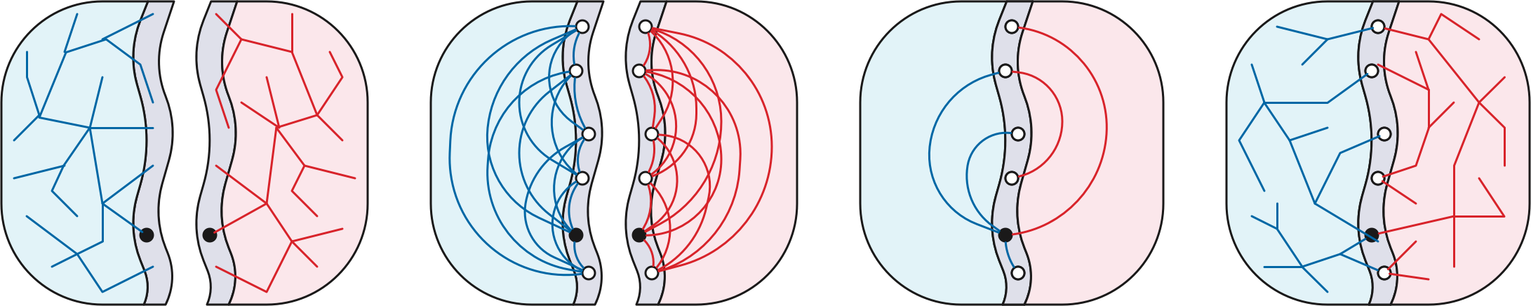
The algorithm starts by computing a balanced cycle separator \(S\) for \(\Sigma\). Let \(A\) and \(B\) be the pieces of \(\Sigma\) obtained by slicing along \(S\), and let \(r\) be any vertex in \(S\). The algorithm has five stages.
Recursively compute \(\textsf{dist}_A(r, A)\) and \(\textsf{dist}_B(r, B)\). How the Recursion Fairy does this is none of your business.
Compute \(\textsf{dist}_A(S, S)\) and \(\textsf{dist}_B(S, S)\). Because \(S\) is a simple cycle, we can compute all separator-to-separator distances within each piece time using either of our multiple-source shortest-path algorithms. There are \(O(n)\) vertices in each piece, and we want to compute \(k = |S|^2 = O(n)\) boundary-to-boundary distances within each piece, so our MSSP algorithms run in \(O(n\log n + k\log n) = O(n\log n)\) time.7
Compute \(\textsf{dist}_\Sigma(r, S)\). Build a complete directed graph \(\hat{S}\) with vertices \(S\), where each dart \(u \mathord\to v\) has length \(\min \{ \textsf{dist}_A(u,v), \textsf{dist}_B(u,v) \}\). The graph \(\hat{S}\) has \(O(\sqrt{n})\) vertices and \(O(n)\) edges, so we can compute \(\textsf{dist}_\Sigma(r, S) = \textsf{dist}_{\hat{S}}(r, S)\) using Bellman-Ford in \(O(r^{3/2})\) time.
Compute \(\textsf{dist}_\Sigma(r, \Sigma)\) using Johnson’s repricing trick. We construct a graph \(H\) from the disjoint union \(A\sqcup B\) as follows. First we add an artificial source vertex \(\hat{r}\). Then for each separator vertex \(v\in S\), we add directed edges \(\hat{r}\mathord\to v_A\) and \(\hat{r}\mathord\to v_B\) to the copies of \(v\) in \(A\) and \(B\), both with length \(\textsf{dist}_\Sigma(r, v)\), which we computed in step 3. For any target vertex \(t\), we have \(\textsf{dist}_\Sigma(r, t) = \textsf{dist}_H(\hat{r}, t)\). Now we define prices for the vertices of \(H\) using the distances we computed in step 2: \[ \pi(v) = \begin{cases} \textsf{dist}_A(r, v) & \text{if $v$ is a vertex of $A$} \\ \textsf{dist}_B(r, v) & \text{if $v$ is a vertex of $B$} \\ \infty & \text{if $v = \hat{r}$.} \end{cases} \] Here \(\infty\) is a symbolic placeholder for some sufficiently large value.8 Straightforward calculation implies that all darts in \(H\) have non-negative repriced length. \(H\) is a planar graph with \(O(n)\) vertices and edges, so we can compute shortest paths in \(H\) in \(O(n\log n)\) time via Dijkstra’s algorithm, or in \(O(n\log\log n)\) time using our faster algorithm based on \(r\)-divisions.9
The overall running time \(O(n^{3/2})\) is dominated by the application of Bellman-Ford in stage 3. Any further improvements require speeding up Bellman-Ford, which is exactly what we’re going to do next!
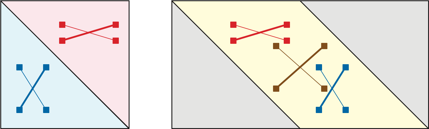
A two-dimensional array \(M\) is Monge if \[ M[i, j] + M[i’, j’] \le M[i, j’] + M[i’, j] \] for all array indices \(i<i’\) and \(j<j’\). Monge arrays are named after the French geometer and civil engineer Gaspard Monge, who described an equivalent geometric condition in his 1781 Mémoire sur la Théorie des Déblais et des Remblais. Monge observed that if \(A, B, b, a\) are the vertices of a convex quadtrilateral in cyclic order, the triangle inequality implies that \(|Aa| + |Bb| < |Ab| + |aB|\).

In 1987, Alok Aggarwal, Maria Klawe, Shlomo Moran, Peter Shor, and Robert Wilber described an elegant recursive algorithm that finds the minimum element in every row of an \(n\times n\) Monge array in \(O(n)\) time, now usually called the SMAWK algorithm after the suitably-permuted initials of its authors. In 1990, Maria Klawe and Daniel Kleitman described an extension to the SMAWK algorithm that finds row-minima in partial Monge matrices, where some entries are undefined, but the Monge inequality holds whenever all four entries are defined. Klawe and Kleitman’s algorithm runs in \(O(n\,\alpha(n))\) time, where \(\alpha(n)\) is the slowly-growing inverse Ackermann function. Very recently, Timothy Chan described a randomized algorithm that find all row-minima in a staircase-Monge matrix in \(O(n)\) expected time.
A description of these algorithms is beyond the scope of this class, but you can find a complete description and analysis of the basic SMAWK algorithm in my algorithms lecture notes.
In the same 2001 paper where they defined dense distance graphs, Fakcharoenphol and Rao described how to use SMAWK to compute shortest paths in planar maps more quickly.
Let \(\Sigma\) be a planar map with weighted edges. Let \(s_1, s_2, \dots, s_k\) be the sequence of vertices on the boundary of the outer face of \(\Sigma\), in cyclic order. (If the outer face boundary is not a simple cycle, the same vertex may appear multiple times in this list.) Let \(D\) be the \(k\times k\) array where \(D[i,j] = \textsf{dist}_\Sigma(s_i, s_j)\).
It follows that the Monge inequality \[ M[i, j] + M[i’, j’] \le M[i, j’] + M[i’, j]; \] holds for any indices \(i, i’, j, j’\) that appear in that cyclic order (possibly with ties) modulo \(k\). In particular, the Monge inequality holds whenever \(i\le i’\le j\le j’\), which implies that the portion of \(M\) on or below the main diagonal is Monge. Symmetrically, the portion of \(M\) on or above the main diagonal is Monge. These two partial Monge matrices cover \(M\). \(\qquad\square\)
Perhaps a better way to express this analysis is that the \(k\times 2k\) partial array defined by \[ D[i,j] := \begin{cases} \textsf{dist}_G(s_i, s_{j \bmod k}) & \text{if $i\le j\le i+k$} \\ \text{undefined} & \text{otherwise} \end{cases} \] is a single partial Monge array.
Now recall that the third phase of our nested-dissection algorithm computes the distances \(\textsf{dist}_\Sigma(r, S)\) by running Bellman-Ford on a weighted directed clique \(\hat{S}\) over the vertices in \(S\). Let \(s_1, s_2, \dots, s_k\) denote the vertices of the cycle separator \(S\), in order around the cycle. It will be more convenient to think of \(\hat{S}\) as the overlay of two directed cliques \(\hat{S}_A\) and \(\hat{S}_B\), in which each edge \(s_i\mathord\to s_j\) has lengths \(\ell_A(s_i\mathord\to s_j) = \textsf{dist}_A(s_i, s_j)\) and \(\ell_B(s_i\mathord\to s_j) = \textsf{dist}_B(s_i, s_j)\), respectively.
The Bellman-Ford algorithm has the following simple structure. After initializing \(\textsf{dist}[r] = 0\) and \(\textsf{dist}[v] = \infty\) for all \(v\ne r\), the algorithm repeatedly identifies and then relaxes all tense edges in \(\hat{S}\). The algorithm terminates after \(O(k)\) relaxation phases, where \(k = O(\sqrt{n})\) is the number of vertices in \(S\).
Here is some pseudo-Python for a single relaxation phase:
for i in range(k):
    for j in range(k):
        if dist[j] < dist[i] + l[i,j]
            dist[j] = dist[i] + l[i,j]
As written, this block of code runs in \(O(k^2)\) time. Because the order that we scan the edges doesn’t matter, let’s first scan all edges in \(\hat{S}_A\) and then all edges in \(\hat{S}_B\):
for i in range(k):
    for j in range(k):
        if dist[j] < dist[i] + lA[i,j]
            dist[j] = dist[i] + lA[i,j]
for i in range(k):
    for j in range(k):
        if dist[j] < dist[i] + lB[i,j]
            dist[j] = dist[i] + lB[i,j]
Now I’m going to do something a little weird to the first block of
code. For each vertex \(v\), I’ll first
figure out the minimum value of dist[i] + lA[i,j] and only
compare that minimum value to dist[j] at the end.
for j in range(k):
    bestcost = math.inf
    for i in range(k):
        if dist[i] + lA[i,j] < bestcost:
            best[j] = i
            bestcost = dist[i] + lA[i,j]
for j in range(k):
    if dist[j] < bestcost:
        dist[j] = bestcost
The first (outer) for-loop is choosing the minimum element in every
column of a \(k\times k\)
matrix \(M\), where \[
M[i,j] := \textsf{dist}(s_i) + \textsf{dist}_A(s_i, s_j)
\] \(M\) is the sum of a matrix
with constant columns (which is Monge) and the boundary-to-boundary
distance matrix in \(A\). Thus, \(M\) can be split into two partial Monge
arrays, and therefore so can its transpose. It follows that we can
compute best[j] (and therefore dist[j]) for
all \(j\) in \(O(k\alpha(k))\) time using Klawe and
Kleitman’s algorithm, or in \(O(k)\)
expected time using Chan’s algorithm.
The same modification relaxes every tense edge in \(\hat{S}_B\) in \(O(k\alpha(k))\) time, or \(O(k)\) expected time.
With this optimization in place, Bellman-Ford computes all shortest-path distances \(\textsf{dist}_\Sigma(r, S)\) in \(O(k) \cdot O(k\alpha(k)) = O(n\alpha(n))\) time, or in \(O(n)\) expected time. This accelerated version of Bellman-Ford is now commonly called “FR-Bellman-Ford” after Fakcharoenphol and Rao, who described a similar but slightly slower reduction to the original SMAWK algorithm.[^fr]
With all these improvements in place, we obtain a shortest-path algorithm described by Philip Klein, Shay Mozes, and Oren Weimann in 2009.
The overall running time satisfies the recurrence \[ T(n) \le T(n_A) + T(n_B) ~+~ O(n\log n) \] where (after a suitable domain transformation) \(n_A + n_B = n\) and \(\max\{n_A, n_B\} \le 3n/4\). We conclude that the algorithm runs in \(O(n\log^2 n)\) time; our invocation of MSSP in stage 2 is (just barely) the bottleneck.
In 2010, Shay Mozes and Christian Wulff-Nilsen improved this algorithm even further by using a good \(r\)-division at each level of recursion (with \(r \approx n/\log n\)) instead of just one separator cycle; their improved algorithm runs in \(O(n\log^2n /\log\log n)\). I will describe their improvement at the end of the next lecture note.
Alok Aggarwal, Maria M. Klawe, Shlomo Moran, Peter Shor, and Robert Wilber. Geometric applications of a matrix-searching algorithm. Algorithmica 2(1–4):195–208, 1987. The SMAWK algorithm.
Noga Alon and Raphael Yuster. Solving linear systems through nested dissection. Proc. 51st IEEE Symp. Found. Comput. Sci., 225–234, 2010.
Bernard A. Carré. An algebra for network routing problems. IMA J. Appl. Math. 7(3):273–294, 1971.
Timothy M. Chan. (Near-)linear-time randomized algorithms for row minima in Monge partial matrices and related problems. Proc. 32nd Ann. ACM-SIAM Symp. Discrete Algorithms, 1465–1482, 2021.
Jack Edmonds and Richard M. Karp. Theoretical improvements in algorithmic efficiency of network flow problems. J. Assoc. Comput. Mach. 19(2):248–264, 1972.
Jittat Fakcharoenphol and Satish Rao. Planar graphs, negative weight edges, shortest paths, and near linear time. J. Comput. Syst. Sci. 72(5):868–889, 2006.
Greg N. Frederickson. Fast algorithms for shortest paths in planar graphs with applications. SIAM J. Comput. 16(8):1004–1004, 1987.
Alan George. Nested dissection of a regular finite element mesh. SIAM J. Numer. Anal. 10(2):345–363, 1973.
Monika R. Henzinger, Philip Klein, Satish Rao, and Sairam Subramanian. Faster shortest-path algorithms for planar graphs. J. Comput. Syst. Sci. 55(1):3–23, 1997.
Carl Gustav Jacob Jacobi. De aequationum differentialum systemate non normali ad formam normalem revocando (Ex Ill. C. G. J. Jacobi manuscriptis posthumis in medium protulit A. Clebsch). C. G. J. Jacobi’s gesammelte Werke, fünfter Band, 485–513, 1890. Bruck und Verlag von Georg Reimer. English translation in [8].
Carl Gustav Jacob Jacobi and François Ollivier (translator). The reduction to normal form of a non-normal system of differential equations. Appl. Algebra Eng. Commun. Comput. 20(1):33–64, 2009. English translation of [7].
Donald B. Johnson. Efficient algorithms for shortest paths in sparse networks. J. Assoc. Comput. Mach. 24(1):1–13, 1977.
Maria M. Klawe and Daniel J. Kleitman. An almost linear time algorithm for generalized matrix searching. SIAM J. Discrete Math. 3(1):81–97, 1990.
Philip Klein, Shay Mozes, and Oren Weimann. Shortest paths in directed planar graphs with negative lengths: A linear-space \(O(n \log^2 n)\)-time algorithm. ACM Trans. Algorithms 6(2):30:1–30:18, 2010.
Richard J. Lipton, Donald J. Rose, and Robert Endre Tarjan. Generalized nested dissection. SIAM J. Numer. Anal. 16:346–358, 1979.
Kurt Mehlhorn and Bernd H. Schmidt. A single shortest path algorithm for graphs with separators. Proc. 4th Int. Conf. Foundations of Computation Theory, 302–309, 1983. Lecture Notes Comput. Sci. 158, Springer.
Gaspard Monge. Mémoire sur la théorie des déblais et des remblais. Histoire de l’Académie royale des sciences 666–705, 1781.
Shay Mozes and Christian Wulff-Nilsen. Shortest paths in planar graphs with real lengths in \(O(n \log^2 n/\log\log n)\) time. Proc. 18th Ann. Europ. Symp. Algorithms, 206–217, 2010. Lecture Notes Comput. Sci. 6347, Springer-Verlag. arXiv:0911.4963.
Siamak Tazari and Matthias Müller-Hannemann. Shortest paths in linear time on minor-closed graph classes, with an application to Steiner tree approximation. Discrete Appl. Math. 157(4):673–684, 2009.
Nobuaki Tomizawa. On some techniques useful for solution of transportation network problems. Networks 1:173–194, 1971.
If we are given the shortest-path tree rooted at any boundary vertex, the remainder of the parametric MSSP algorithm runs correctly, without modification, in \(O(n\log n)\) time.↩︎
In particular, the original graph \(G\) contains a negative cycle if and only if, at after eliminating some subset of vertices, \(G\) contains an edge \(xy\) such that \(\ell(x{\to}y) + \ell(y{\to}x) < 0\).↩︎
I’m playing a little fast and loose here. Recall that the Klein-Mozes-Sommer separator hierarchy does not necessarily evenly partition vertices at every level of recursion, but only at every third level. So formalizing this analysis requires considering eight recursive subproblems, not just two.↩︎
The formulation of optimal path problems as solving linear systems over \((\min,+)\)- and \((\max,+)\)-algebras dates back to at least the 1960s. For example, in 1971 Bernard Carré observed that different formulations of Bellman-Ford are \((\min,+)\)-variants of Jacobi and Gauss-Seidel iteration, and the Floyd-Warshall all-pairs shortest-path algorithm is a \((\min,+)\)-variant of Jordan elimination.↩︎
Specifically, Lipton, Rose, and Tarjan’s elimination algorithm assumes that when a row is eliminated, its diagonal entry is nonzero. (Recall that the algorithm chooses the elimination order before doing any elimination.) This condition is automatically satisfied for symmetric positive-definition linear systems over \(\mathbb{R}\), but is not satisfied in general.↩︎
At least, first explicitly proposed. Arguably the repricing technique is already implicit in Jacobi’s mid-19th-century description of the “Hungarian” algorithm for the assignment problem.↩︎
Mehlhorn and Schmidt’s algorithm reprices the vertices in each piece, and then runs Dijkstra’s algorithm from each separator vertex, in \(O(n^{3/2}\log n)\) total time.↩︎
If you’re uncomfortable with symbolic infinities, it suffices to set \[ \pi(\hat{r}) = \max\left\{ \textsf{dist}_A(r, u) - \textsf{dist}_\Sigma(r, u), ~ \textsf{dist}_B(r, u) - \textsf{dist}_\Sigma(r, u) \bigm| u\in S \right\} \]↩︎
Mehlhorn and Schmidt compute \(\textsf{dist}_\Sigma(r, \Sigma)\) by brute force in \(O(n^{3/2})\) time, by observing that \(\textsf{dist}_\Sigma(r, v) = \min_{u\in S} \{\textsf{dist}_\Sigma(r, u) + \textsf{dist}_A(u,v)\}\) for every vertex \(v\in A\), and similarly for \(B\).↩︎