
Now let’s generalize the homotopy problem from the last lecture to the case of more than one obstacle. Let \(O = \{a, b, c, \dots\}\) be an arbitrary finite set of points in the plane. The definitions of homotopy and contractible easily generalize to polygons (and other closed curves) in \(\mathbb{R}^2\setminus O\). How quickly can we tell whether two polygons in \(\mathbb{R}^2\setminus O\) are homotopic?
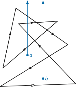
The game Fast and Loose shows some of the subtlety of this problem. Let \(a\) and \(b\) be arbitrarily points in each of the two loops of the curve \(C\) that the con artist actually uses. It’s not hard to see that \(wind(c, a) = wind(C, b) = 0\); any ray upward from either \(a\) or \(b\) has one positive crossing and one negative crossing. Thus, the curve is contractible in the plane with only one of these punctures; in other words, the chain is loose if we only use one finger. But the curve \(C\) is not contractible in \(\mathbb{R}^2 \setminus \{a, b\}\); we can hold the chain fast by placing a finger in each loop. Winding numbers are not a homotopy invariant when there is more than one obstacle.
Just as in the one-obstacle setting, we can (approximately) decompose any homotopy between two polygons in \(\mathbb{R}^2\setminus O\) into safe vertex moves, where now a vertex move is safe if the moving vertex and its incident edges avoids all points in \(O\). Essentially the same argument from the previous lecture implies the following:
However, we can still define a homotopy invariant by shooting rays out of every obstacle, and recording how the polygon intersects these rays. Specifically, we record not only the number of times the polygon crosses each ray, but the actual order and directions of these crossings.
As usual, we will assume without loss of generality that the obstacles have distinct \(x\)-coordinates. Shoot a vertical ray upward from each obstacle point; I’ll call these vertical rays fences. The crossing sequence of a polygon \(P\) in \(\mathbb{R}^2\setminus O\) is the sequence of intersections between the fences and the polygon, in order along the polygon, along with the sign of each crossing (positive if the polygon crosses the fence to the left, negative if the polygon crosses the fence to the right).
Figure 2 shows a polygon in the plane with two obstacle points \(a\) and \(b\). If we orient the polygon as indicated
by the arrows, starting at the lower left corner, the crossing sequence
is BAabBAabB, where each upper-case letter
denotes a positive crossing through the corresponding fence, and each
lower-case letter denotes a negative crossing through the corresponding
fence.
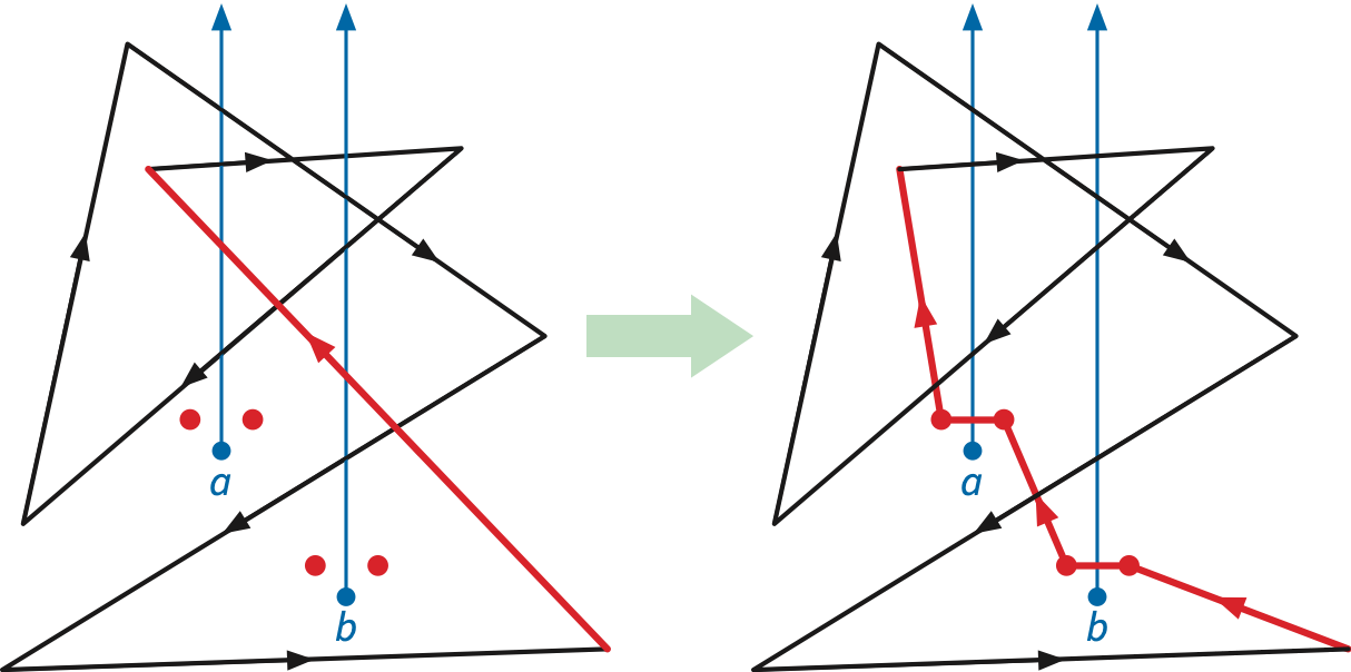
First, we define two new sentinel points \(a^\flat\) and \(a^\sharp\) just above and on either side of each obstacle \(a\). These points are close enough to \(a\) that no vertex of \(P\), no other obstacle, and no other sentinel point lies on or between the vertical lines through \(a^\flat\) and \(a^\sharp\).
Next, we divert edges through the sentinel points, by adding two additional vertices near each intersection between \(P\) and any fence, and then moving those new vertices to the sentinel points near the corresponding obstacle.
Finally, we divert the rest of the polygon to a single point far below any obstacle. First we add a new vertex at the midpoint of each edge of \(P'\) between two sentinel points of different obstacles. Then we choose a point \(z\) sufficiently far below the polygon and the sentinel points that for any polygon vertex \(p\), the segment \(zp\) does not cross any of the fences. Finally, we move every vertex of \(P'\) that is not a sentinel point directly to this new bottom point \(z\). Again, this deformation does not change the polygon’s crossing sequence.
The resulting canonical polygon \(P''\) is a concatenation of loops of the form \(z a^\flat a^\sharp z\) (for each negative crossing) or \(z a^\sharp a^\flat z\) (for each positive crossing).
Unfortunately, the converses of these two results are false; a homotopy that moves one polygon vertex across one fence either inserts or deletes a pair of crossings in the polygon’s crossing sequence. Thus, crossing sequences are not homotopy invariants. Fortunately, this is the only way that a homotopy can change the crossing sequence.
We regard signed crossing sequences as strings of abstract symbols, where each symbol \(a\) has a formal “inverse” \(\bar{a}\). In our earlier example, each upper case letter is the inverse of the corresponding lower-case letter, and vice versa. Let \(x\cdot y\) denote the concatenation of strings \(x\) and \(y\), and let \(\varepsilon\) denote the empty string.
An elementary reduction is a transformation of the form \(x\cdot a\bar{a}\cdot y \mapsto x\cdot y\), where \(x\) and \(y\) are (possibly empty) strings and \(a\) is a single symbol. An elementary expansion is the reverse transformation \(x\cdot y \mapsto x\cdot a\bar{a}\cdot y\). Two strings are equivalent if once can be transformed into the other by a sequence of elementary reductions and expansions. (Check for yourself that equivalence is in fat an equivalence relation!) We call a string trivial if it is equivalent to the empty string \(\varepsilon\). Finally, a string is reduced if no elementary reductions are possible; for example, the empty string \(\varepsilon\) is trivially reduced, as is any string of length \(1\).
Crossing sequences of polygons are actually cyclic strings.
Formally, a cyclic string is an equivalence class of linear strings:
\[
(w) := \{ y\cdot x \mid x\cdot y = w \}
\] For example, (ABbA) = {ABbA,
BbAA, bAAB, AABb} and \((\varepsilon) = \{\varepsilon\}\). I’ll
write \(w \sim z\) to denote that \(w\) is a cyclic shift of \(z\), or equivalently \(w\in(z)\), or equivalently \(z\in (w)\). To emphasize that elementary
reductions can “wrap around” cyclic strings, we say that a cyclic string
is cyclically reduced if no elementary reductions are possible.
A (cyclic) string is trivial if it is equivalent to the empty
(cyclic) string.
For example, the cyclic string
(EcaCbaABcEeEeAdbcCBaEdDeADCe) is trivial; two different
sequences of elementary reductions are shown below (using interpuncts to
represent missing symbols). In the first sequence, each elementary
reduction removes the leftmost matching pair; the second
sequence is more haphazard. In fact, as the following lemma implies,
any sequence of elementary reductions eventually reduces this
string to nothing.
EcaCbaABcEeEeAdbcCBaEdDeADCe
EcaCb··BcEeEeAdbcCBaEdDeADCe
EcaC····cEeEeAdbcCBaEdDeADCe
Eca······EeEeAdbcCBaEdDeADCe
Eca········EeAdbcCBaEdDeADCe
Eca··········AdbcCBaEdDeADCe
Ec············dbcCBaEdDeADCe
Ec············db··BaEdDeADCe
Ec············d····aEdDeADCe
Ec············d····aE··eADCe
Ec············d····a····ADCe
Ec············d··········DCe
Ec························Ce
E··························e
····························
EcaCbaABcEeEeAdbcCBaEdDeADCe
EcaCbaABcEeEeAdb··BaEdDeADCe
EcaCb··BcEeEeAdb··BaEdDeADCe
·caCb··BcEeEeAdb··BaEdDeADC·
·caC····cEeEeAdb··BaEdDeADC·
·caC····cE··eAdb··BaEdDeADC·
·caC····cE··eAdb··BaE··eADC·
·caC····cE··eAdb··Ba····ADC·
·caC····cE··eAd····a····ADC·
··aC····cE··eAd····a····AD··
··aC····c····Ad····a····AD··
··aC····c····Ad··········D··
··a··········Ad··········D··
··a··········A··············
····························It follows that applying only elementary reductions leads to a unique reduced string; however, equivalence also allows elementary expansions. Consider two equivalent but distinct cyclic strings \(x\ne y\), and let \(x = w_1 \leftrightarrow w_2 \leftrightarrow \cdots \leftrightarrow w_n = y\) be a sequence of strings, each connected to its success by an elementary reduction in one direction \(w_i \mapsto w_{i+1}\) or the other \(w_{i+1} \mapsto w_i\).
Suppose for some index \(i\), we have reductions \(w_i \mapsto w_{i-1}\) and \(w_i \mapsto w_{i+1}\). If \(w_{i-1} = w_{i+1}\), then we can remove \(w_{i-1}\) and \(w_i\) to obtain a shorter transformation sequence. Otherwise, there is another string \(z_i\) such that \(w_{i-1}\mapsto z_i\) and \(w_{i+1} \mapsto z_i\). Thus, by induction, we can modify our transformation sequence so that every reduction appears before every expansion.
Let \(z\) be the shortest string in this normalized sequence. Both \(x\) and \(y\) can be reduced to \(z\) using only elementary reductions. Because \(x\ne y\), either \(x \ne z\) or \(y\ne z\); we conclude that at most one of \(x\) and \(y\) is reduced.
X is
an array of non-zero integers, with inverses indicated by negation. The
algorithm runs in two phases. The first phase reduces the
linear sequence \(X\) by
repeatedly removes the leftmost matching pair, using the output array as
a stack. The second phase performs any remaining cyclic reductions that
“wrap around” the ends of the array.
def LeftGreedyReduce(X):
    n = size(X)
    Y = [0] * n                             // reduced sequence = stack
    top = -1                                // top stack index
    // ————— linear reduction —————
    for i in range(n):
        if top < 0 || (X[i] != -Y[top]):    // empty or no match
            top = top + 1
            Y[top] = X[i]                   // push
        else:
            top = top - 1                   // pop
    // ————— cyclic reduction —————
    bot = 0
    while (bot < top) and (Y[bot] = -Y[top]):
        bot = bot + 1
        top = top - 1
    // ————— done! —————
return Y[bot:top+1]Conversely, any elementary reduction of the signed crossing sequence can be modeled by a sequence of safe vertex moves, performed either directly on the original polygon or (more easily) on the canonical polygon with the same crossing sequence.
We finally have all the ingredients of our homotopy-testing algorithm.
Let me emphasize here that the algorithm does not construct an explicit homotopy between the two polygons.
To be written
Polygons with holes: Replace each hole with a sentinel point.
Paths: