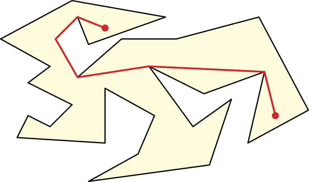
In this lecture, we’ll consider a problem that combines both geometry and topology that arises in VLSI design (or at least did arise in VLSI design in the 1980s). Suppose we have an environment \(X\) that can be modeled as a polygon with holes; this is the area bounded between a simple outer polygon \(P_0\) and several disjoint simple polygons or “holes” \(P_1, P_2, \dots, P_h\), each of which lies in the interior of \(P_0\). (Yes, previously we used “polygon” to refer to the boundary, and now we’re using “polygon with holes” to refer to the area. Welcome to mathematical jargon.)
We are also given a polygonal path \(\pi\) in the interior of \(X\). Recall that two paths are homotopic if one can be continuously deformed to the other within \(X\) while keeping both endpoints fixed at all times. Our problem is to find the shortest path (that is, the path of minimum Euclidean length) that is homotopic in \(X\) to the given path \(\pi\).
Although we could reduce to our earlier notion of homotopy by using the vertices of \(X\) as point obstacles, the pictures will be nicer (and the algorithms arguably simpler) if we use \(X\) itself as our underlying space. Our earlier formal definition of homotopy extends directly to this setting: A homotopy between two paths \(\alpha\) and \(\beta\) in \(X\) is a continuous function \(h\colon[0,1]\times[0,1]\to X\) such that the restrictions \(h(\cdot,0)\) and \(h(\cdot,1)\) are constant functions, and the restrictions \(h(0,\cdot)\) and \(h(1, \cdot)\) are the paths \(\alpha\) and \(\beta\), respectively.
Throughout this section, \(n\) denotes the number of vertices of the environment \(X\), and \(k\) denotes the number of vertices in the input path \(\pi\). (Yes, this is reversed from the previous lecture.) Let \(s\) (“source”) and \(t\) (“target”) denote the first and last vertices of \(\pi\).
Let’s start with the topologically trivial case where \(X\) is the interior of a simple polygon with no holes. A strengthening of the Jordan Curve Theorem due to Schönflies implies that \(X\) is homeomorphic to an open circular disk. It follows that any two paths in \(X\) with the same endpoints are homotopic. Thus, we are now looking for the globally shortest path in \(X\) between the endpoints of \(\pi\).
The shortest path between two points \(s\) and \(t\) in a simple polygon \(P\) is a polygonal chain, whose interior vertices lie at concave vertices of \(P\). Imagine a taut rubber band between \(s\) to \(t\); the rubber band will be straight everywhere, except at concave corners that it must wrap around.
I’ll describe an algorithm for this special case as through the topology of the problem were non-trivial; in particular, even though the output depends only on the endpoints of the input path \(\pi\), I will still use the entire input path to guide the algorithm.
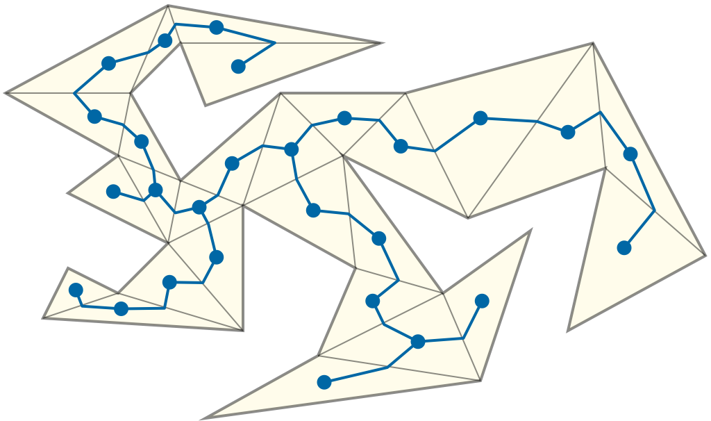
The first step of our shortest-path algorithm is to triangulate the polygon \(X\). We saw an algorithm in the first lecture that computes a frugal triangulation of \(X\) in \(O(n\log n)\) time.
The (weak) dual graph of a polygon triangulation has a vertex for each triangle and an edge for each diagonal; two vertices are connected by an edge in the dual graph if and only if the corresponding triangles share a diagonal. We can draw the dual graph by placing each vertex at the centroid of its triangle, and drawing each edge as a polygonal path through the midpoint of the corresponding diagonal.
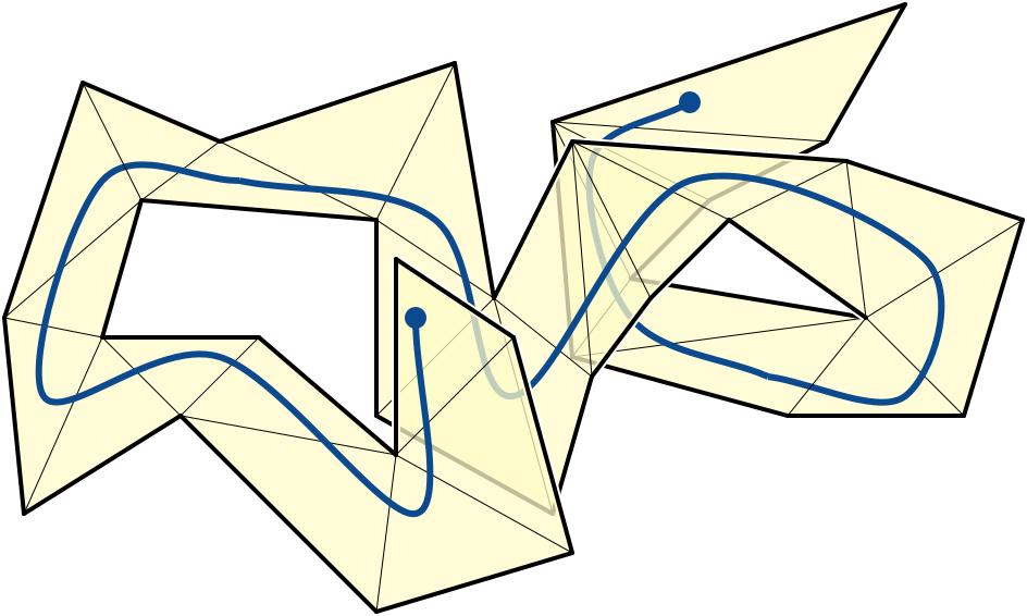
Next we apply the same strategy that we previously used to test contractibility. We compute the crossing sequence of \(\pi\) and then reduce it as much as possible. (Two paths are homotopic if and only if they have identical reduced crossing sequences.) In this setting, the crossing sequence is the sequence of diagonals crossed by \(\pi\), in order along \(\pi\).

In our earlier homotopy-testing algorithm, we also recorded the
sign of each crossing, but that information is actually
redundant in our current setting. Recall from our proof of the polygon
triangulation theorem that any interior diagonal partitions the interior
of a polygon into two disjoint subsets. Thus, if \(\pi\) crosses the same diagonal multiple
times, those crossings must alternate between positive and negative. It
also follows that we can reduce the crossing sequence by removing
arbitrary adjacent pairs of equal symbols; for any such pair,
the corresponding crossings have opposite signs. For example, the
crossing sequence
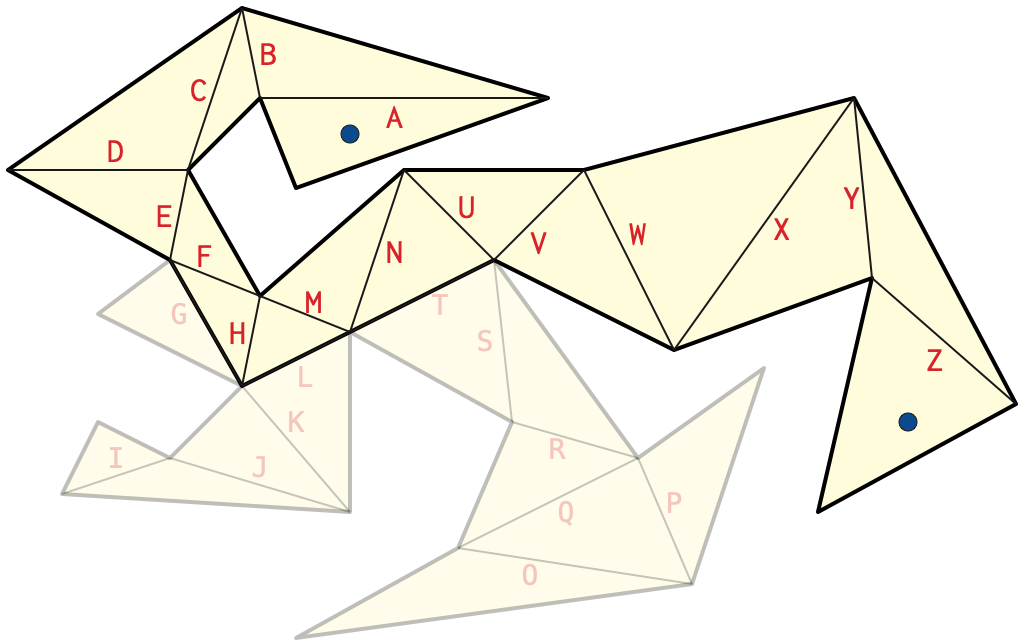
ABCDDDEFHLKJJKLMNUUTSRQPPQQOOQRSTUVWWWXYYXXYZ of the path
in the previous figure reduces to ABCDEFHMNUVWXYZ.
We can compute the crossing sequence of \(\pi\) in \(O(n + k + x)\) time, where \(x = O(kn)\) is the length of the crossing sequence. Specifically, we find the triangle containing \(s\) by brute force; then we can repeatedly find the next crossing (if any) along the current edge of \(\pi\) in \(O(1)\) time. Finally, we can reduce the crossing sequence in \(O(x)\) time using left-greedy cancellation.
(The reduced crossing sequence of \(\pi\) contains precisely the edge labels that appear an odd number of times in the unreduced crossing sequence; moreover, these labels appear in the same order as their first (or last) occurrences in the unreduced crossing sequence.)
Let \(\bar{x}\) denote the length of the reduced crossing sequence. The reduced crossing sequence defines a sequence of \(\bar{x}+1\) triangles in the triangulation of \(X\), starting with the triangle containing the first vertex \(\pi_0\) of \(\pi\), and ending with the triangle containing the last vertex \(\pi_k\) of \(\pi\). The union of these triangles is called the sleeve of the reduced crossing sequence.
Any path \(\alpha\) in \(X\) from \(s\) to \(t\) that leaves the sleeve must cross a diagonal \(d\) on the boundary of the sleeve. The endpoints \(s\) to \(t\) lie in the same component of \(X\setminus d\), so the path must cross \(d\) and even number of times. Let \(p\) and \(q\) be the first and last intersection points along \(\alpha\). The line segment \(pq\) is shorter than the subpath of \(\alpha\) from \(p\) to \(q\), so \(\alpha\) cannot be a shortest path.
Alternatively, the crossing sequence describes a walk in the dual graph of the triangulation, starting at the vertex dual to the triangle containing \(s\). Reducing the crossing sequence removes spurs from this walk—subpaths that consist of the same edge twice in a row, necessarily in opposite directions. Thus, the reduced crossing sequence describes a shortest walk—in fact, the unique simple path between its endpoints—in the dual graph. This path is also the dual graph of the induced triangulation of the sleeve.
Note that we do not actually need to construct the sleeve; the sequence of diagonals that the funnel crosses is exactly the reduced crossing sequence of \(\pi\).
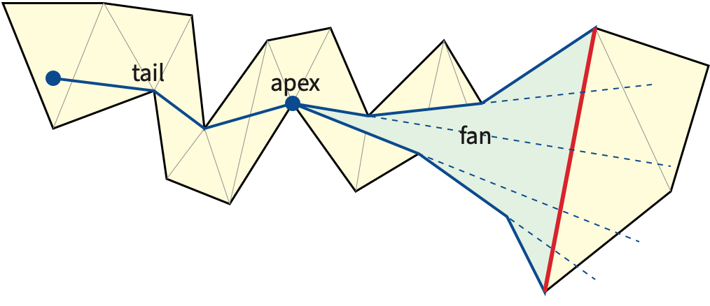
To compute the actual shortest path from \(s\) to \(t\), we use an algorithm independently discovered by Tompa (1981), Chazelle (1982), Lee and Preparata (1984), and Leiserson and Maley (1985). (My presentation most closely follows Lee and Preparata’s.) The funnel of any diagonal \(d\) of the sleeve is the union of the shortest paths the from the source point \(s\) to all points on \(e\).
The funnel consists of a polygonal path, called the tail, from \(s\) to a point a called the apex, plus a simple polygon called the fan. The tail may be empty, in which case \(s\) is the apex. The fan is bounded by the diagonal \(d\) and two concave chains joining the apex to the endpoints of \(d\). The shortest path from \(s\) to either endpoint of \(d\) consists of the tail plus one of the concave chains bounding the fan. Extending the edges of the concave chains to infinite rays defines a series of wedges, which subdivide both the fan and the triangle just beyond \(d\).
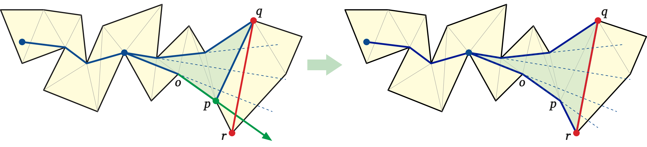
Beginning with a single triangle joining \(s\) to the first edge in the reduced crossing sequence, we extend the funnel through the entire sleeve one diagonal at a time. Each diagonal in the sleeve shares one endpoint with the previous diagonal; suppose we are extending the funnel from diagonal \(pq\) to diagonal \(qr\). Let \(o\) be the predecessor of \(p\) on the shortest path from \(s\) to \(p\).
There are two cases to consider, depending on whether \(q\) and \(r\) lie on the same sides of the line through \(o\) and \(p\) or on opposite sides. We can actually detect this case in \(O(1)\) time with a single orientation test.
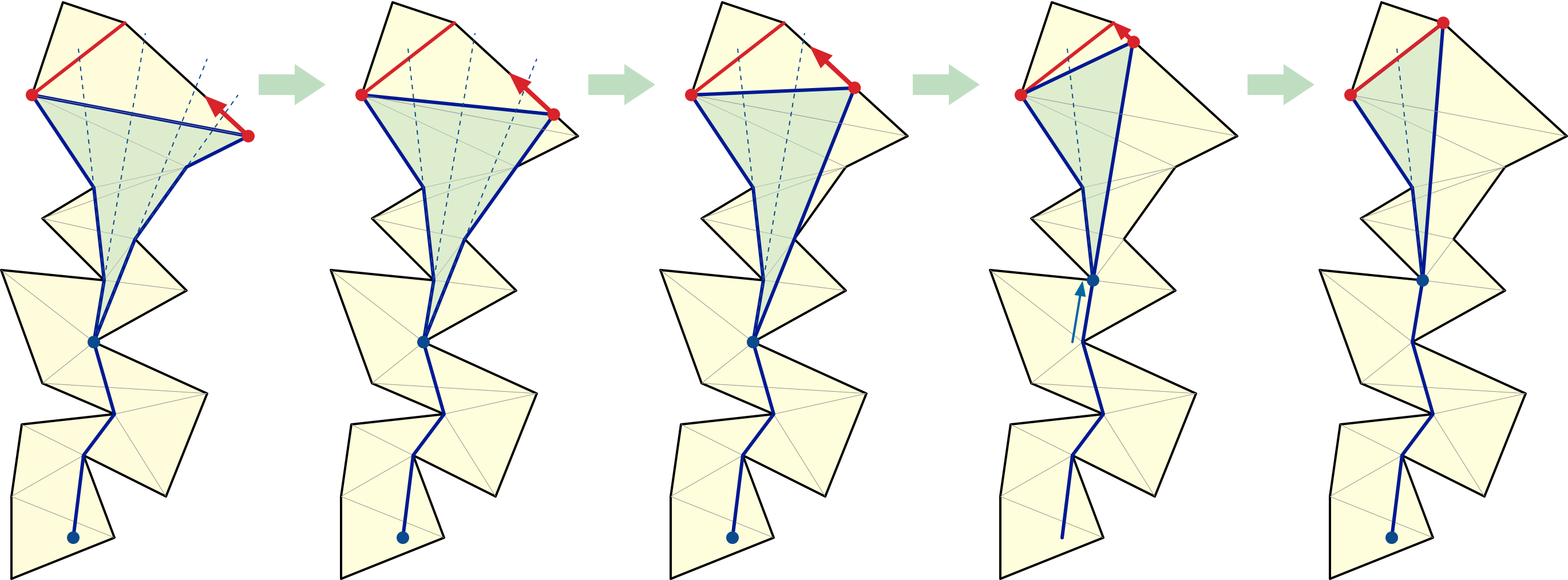
Let \(yz\) be the last diagonal in the reduced crossing sequence. To end the algorithm, we treat the line segment \(tz\) as another diagonal and extend the funnel one more time. The shortest path homotopic to \(\pi\) then consists of the tail of the funnel plus the concave chain of the fan containing \(t\); we can extract this shortest path in \(O(1)\) time per edge.
Summing up, we spend \(O(n\log n)\) time triangulating \(X\), then \(O(k+x) = O(nk)\) time computing the crossing sequence of \(\pi\), then \(O(x) = O(nk)\) time reducing the crossing sequence, \(O(\bar{x}) = O(nk)\) time growing the funnel, and finally \(O(\bar{x}) = O(nk)\) extracting the shortest path from the final funnel.
Now let’s consider the more general case where \(X\) has one or more holes. Perhaps surprisingly, the previous algorithm needs no modifications whatsoever to compute the shortest path homotopic to \(\pi\) in \(O(n\log n + nk)\) time.
Triangulate \(X\) in \(O(n\log n)\) time using the algorithm described in the first lecture. First build a trapezoidal decomposition using a sweep-line algorithm (such as Bentley-Ottmann). Then insert diagonals inside every boring trapezoid in \(O(n)\) time, partitioning \(X\) into monotone mountains. Finally, triangulate these monotone mountains in \(O(n)\) total time.
Compute the crossing sequence of \(\pi\) with respect to this triangulation in \(O(n + k + x)\) time, where \(x\) is the number of crossings. Locate the triangle containing \(s\) in \(O(n)\) time by brute force, then repeatedly find the next crossing (if any) along the current edge in \(O(1)\) time.
Reduce the resulting crossing sequence in \(O(x)\) time using the left-greedy reduction algorithm.
Extend the funnel through the sleeve of the reduced crossing sequence in \(O(\bar{x}) = O(nk)\) time using the standard funnel algorithm.
Finally, extract the shortest homotopic path from the final funnel in \(O(1)\) time per edge.
Same algorithm, same running time, same everything. This strikes many people as counterintuitive. After all, the sleeve can runs through the same triangle multiple times, and the funnel can self-intersect; why doesn’t this cause any problems?
One way to answer this question is that the algorithm doesn’t look for self-intersections, so it’s behavior can’t be affected by them. Or said differently: the algorithm only makes local decisions, but self-intersection is a global property. Every branch in our algorithm is based on either a comparison between two \(x\)-coordinates or an orientation test on some triple of points. As far as the algorithm is concerned, every time the funnel enters a triangle, it is entering that triangle for the very first time, or equivalently, it is entering a new copy of that triangle. So the sleeve of the reduced crossing sequence, while not being geometrically a triangulated simple polygon, is still topologically a triangulated simple polygon: a collection of triangles glued together along common edges into a topological disk.
There is a reasonable analogy here with classical graph traversal algorithms: depth-first search, breadth-first search, and their more complex descendants. All of these algorithms maintain a set of vertices; at each iteration, each algorithm pulls one vertex \(v\) out of this set, marks that vertex, and then puts the unmarked neighbors of \(v\) into the set. Without the marking logic, unless the input graph is a tree, these algorithms will visit at least one vertex infinitely many times, each time treating it as a brand-new vertex.
In fact, even the original shortest-path algorithm does not actually require the environment \(X\) to be a simple polygon. We only require that (1) \(X\) is assembled from any set of Euclidean triangles by identifying disjoint pairs of equal-length edges, (2) all triangle vertices are on the boundary of \(X\), and (3) the dual graph of the triangulation is a tree (equivalently, \(X\) is homeomorphic to a disk in the plane). More generally, the shortest-homotopic-path algorithm applies to any triangulated space satisfying conditions (1) and (2); these spaces can reasonably be called boundary-triangulated flat surfaces. For example, without modification, our algorithm can compute shortest homotopic paths on a triangulated Möbius band.
Another explanation that may be more familiar to topologists is that our algorithm is effectively exploring the universal cover of the input polygon. Informally, the universal cover (of universal covering space) of \(X\) is the infinite topological space constructed by a breadth-first search of \(X\) without memory.
We can define the universal cover more constructively in terms of a
triangulation of \(X\) as follows. Fix
a starting point \(s\). For every
reduced crossing sequence \(w\) of a
path starting at \(s\), let \(\Delta_w\) denote an independent
copy of the triangle containing the final point in that path. For
example, \(\Delta_\varepsilon\) is a
copy of the triangle containing \(s\).
Two triangles \(\Delta_w\) and \(\Delta_x\) are neighbors if \(x = wd\) for some diagonal \(d\); glue every such pair together along
their copies of \(d\). For example, if
\(w =\) ABCB and \(x =\) ABCBD, then we would
identify the copies of edge D in \(\Delta_w\) and \(\Delta_x\). We call each triangle \(\Delta_w\) a lift of the
corresponding triangle in the triangulation of \(X\), and we call the original triangle a
projection of \(\Delta_w\).
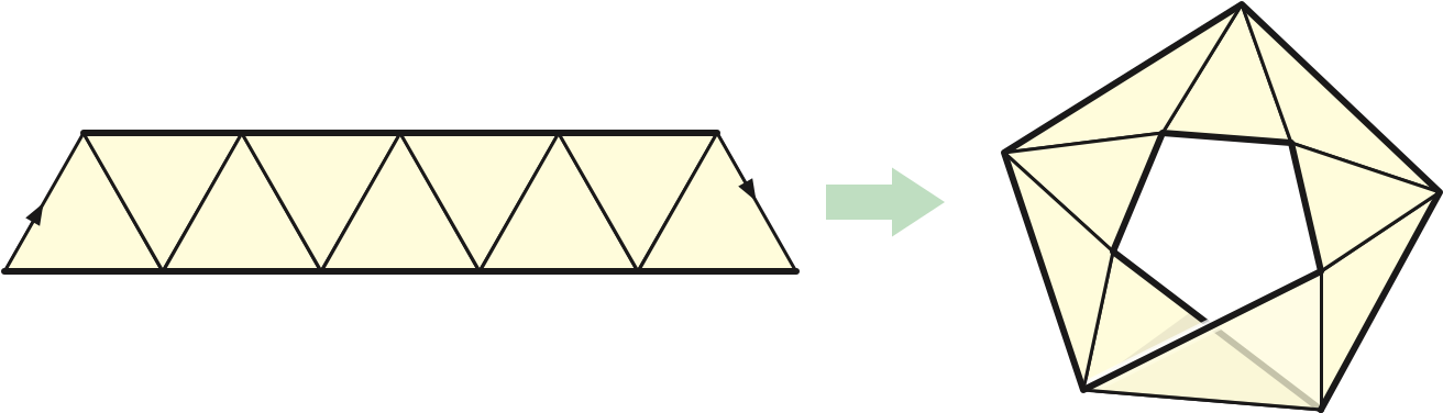
Figure! Polygonal annulus to infinite polygonal parking garage?
The dual graph of the universal cover of \(X\)—or equivalently, the universal cover of the dual graph of \(X\)—has a vertex for every possible reduced crossing sequence (of a path starting at \(s\)), and an edge between two reduced crossing sequences if they differ by exactly one crossing. Unless the input polygon \(X\) has no holes, the universal cover of the dual graph is an infinite tree. The crossing sequence describes a walk from some vertex \(\hat{s}\) to another vertex \(\hat{t}\) in this infinite tree; removing all spurs computes the unique path in that tree between \(\hat{s}\) and \(\hat{t}\).
Figure?
The universal cover is an example of a covering space. We will see several other examples of covering spaces in this course, so let me start here with some formal definitions.
A covering map is a continuous surjective function \(p\colon \widehat{X}\to X\), such that every point \(x\in X\) has an open neighborhood \(U\) whose preimage \(p^{-1}(U)\) is the disjoint union of open sets \(\bigsqcup_{i\in I} U_i\), such that the restriction of the function \(p\) to each open set \(U_i\) is a homeomorphism to \(U\). The open sets \(U_i\) are sometimes called sheets over \(U\). If there is a covering map from \(\widehat{X}\) to \(X\), we call \(\widehat{X}\) a covering space of \(X\). By convention, we require covering spaces to be connected.
The universal covering space \(\widetilde{X}\) can be defined in several different ways:
\(\widetilde{X}\) is the unique covering space of \(X\) that also covers every covering space of \(X\).
\(\widetilde{X}\) is the unique simply-connected covering space of \(X\). (Recall that a space is simply connected if every closed curve in that space is contractible.)
\(\widetilde{X}\) is the space of all homotopy classes of paths from some fixed basepoint \(s\in X\): \[ \widetilde{X} := \big\{ [\pi] \bigm| \pi\colon [0,1]\to X \text{~and~} \pi(0) = s \big\} \] The covering map \(p\colon \widetilde{X}\to X\) maps each homotopy class \([\pi]\) of paths to their common final endpoint \(\pi(1)\).
In our construction by gluing labeled triangles, the covering map sends each triangle \(\Delta_w\) to the corresponding triangle in the triangulation of \(X\).
Concrete examples?
Bernard Chazelle. A theorem on polygon cutting with applications. Proc. 23rd Ann. IEEE Symp. Found. Comput. Sci., 339–349, 1982. The funnel algorithm.
Shaodi Gao, Mark Jerrum, Michael Kaufmann, Kurt Mehlhorn, and Wolfgang Rülling. On continuous homotopic one layer routing. Proc. 4th Ann. Symp. Comput. Geom., 15 392–402, 1988.
John Hershberger and Jack Snoeyink. Computing minimum length paths of a given homotopy class. Comput. Geom. Theory Appl. 4:63–98, 1994.
Der-Tsai Lee and Franco P. Preparata. Euclidean shortest paths in the presence of rectilinear barriers. Networks 14:393–410, 1984. The funnel algorithm.
Charles E. Leiserson and F. Miller Maley. Algorithms for routing and testing routability of planar VLSI layouts. Proc. 17th Ann. ACM Symp. Theory Comput., 69–78, 1985. The funnel algorithm.
Martin Tompa. An optimal solution to a wire-routing problem. J. Comput. System Sci. 23:127–150, 1981. The funnel algorithm.