Recall that a closed curve in the plane is any continuous function from the circle to the plane. Previously we considered a common representation of closed curves as polygons: circular sequences of line segments joined at common endpoints. Polygons are convenient for reasoning about intersections with other simple geometric structures like vertical rays, trapezoidal decompositions, and triangulations, but in other ways the geometry of the representation is irrelevant. Starting with this lecture, I’ll consider a more abstract representation that records only how the curve intersects itself.
A self-intersection \(\gamma(t) = \gamma(t')\) of a closed curve \(\gamma\) is transverse if, for all sufficiently small \(\varepsilon > 0\) the subpaths \(\gamma(t-\varepsilon, t+\varepsilon)\) and \(\gamma(t'-\varepsilon, t'+\varepsilon)\) are homeomorphic to two orthogonal lines. A closed curve is generic if every self-intersection is transverse (in particular, there are no self-tangencies or repeated curve segments) and there are no triple self-intersections \(\gamma(t) = \gamma(t') = \gamma(t'')\).
Two generic curves are isotopic if one can be continuously deformed to the other without ever changing the number of self-intersections. For example, all simple closed curves are isotopic to each other. A homotopy that always preserves the number of self-intersections is called an isotopy. In fact, two planar curves \(\gamma\) and \(\gamma’\) are isotopic if and only if there is an orientation-preserving homeomorphism \(h\colon \mathbb{R}^2 \to \mathbb{R}^2\) such that \(\gamma’ = h\circ \gamma\). At least in the next few lectures, we really don’t care about the geometry of these curves, so we won’t distinguish between isotopic curves.
Generic closed curves are sometimes called immersions or regular curves, but the latter term more commonly refers to closed curves with continuous non-zero derivatives. In fact, the most common word used to describe this class of closed curves is “curve”! The definition of generic curves does not require continuous, non-zero, or even well-defined derivatives at any point, much less at every point. Despite this freedom, the following standard compactness argument implies that generic curves are well-behaved.
Lemma: Every generic closed curve has a finite number of self-intersection points.
The open sets \(\mathcal{C} = \{ U_t \mid t\in S^1 \}\) clearly cover the circle, meaning \(\bigcup_{t\in S^1} U_t = S^1\). Because \(S^1\) is compact, there must be a finite subset \(\mathcal{F} \subset \mathcal{C}\) that also covers \(S^1\). Let \(F \subset S^1\) be the (necessarily finite) index set of the finite subcover \(\mathcal{F}\), meaning \(\mathcal{F} = \{ U_t \mid t\in F \}\).
The only set in \(\mathcal{U}\) that contains a singular point \(t\) is its own interval \(U_t\). Thus, the finite set \(T\) must contain every singular point.
The adjective “generic” is justified by the observation that every closed curve can be approximated arbitrarily closely by a generic closed curve. Previously we argued that every closed curve can be approximated arbitrarily closely by a polygon. (This is the simplicial approximation theorem.) An arbitrarily small perturbation of any polygon ensures that all vertices are distinct, no vertex lies in the interior of an edge, and no three edges share a common point. Any polygon satisfying these conditions is a generic closed curve.
A more careful application of simplicial approximation and compactness implies that any generic closed curve \(\gamma\) can be approximated arbitrarily closely by a polygon that is isotopic to \(\gamma\). Thus, even though generic curves are not polygons by definition, they are polygons without loss of generality. In fact, results in future lectures imply that each generic curve with \(n\) self-intersection points is isotopic to a polygon with only \(O(n)\) vertices.
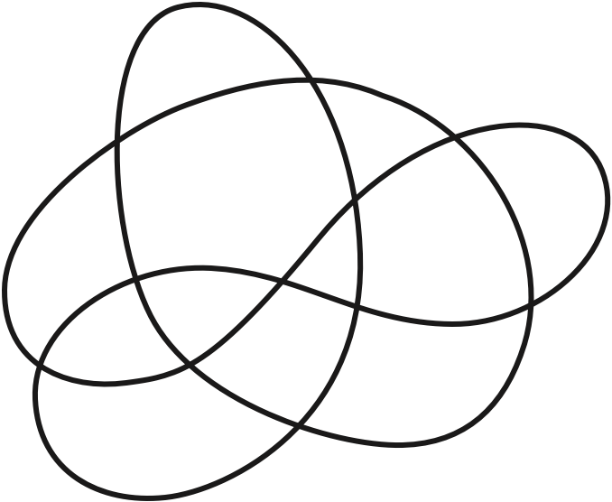
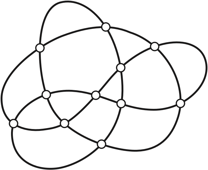
Any non-simple generic closed curve can be naturally represented by its image graph, which is a connected 4-regular plane graph1 whose vertices are the self-intersection points of the curve, and whose edges are curve segments between vertices. Image graphs are not necessary simple; they can contain loops and parallel edges. The image graph of a simple closed curve is obviously a simple cycle.
However, not every 4-regular plane graph is the image graph of a generic closed curve. Any generic curve is a particular Euler tour of its image graph. Recall that an Euler tour of a graph \(G\) is any closed walk that traverses each edge of \(G\) exactly once. A closed walk is Gaussian if, whenever the walk visits a vertex \(v\), it enters and exits \(v\) along opposing edges. A 4-regular graph is unicursal if it contains a Gaussian Euler tour; every unicursal 4-regular plane graph is the image of a non-simple generic curve.
Any generic planar curve partitions the plane into regions called the faces of the curve. The Jordan-Schönflies theorem implies that every planar curve has one unbounded face that is homeomorphic to the complement of a closed disk, and every other face is homeomorphic to an open disk. The faces of a curve are also the faces of its image graph. A face is called a monogon if it has only one edge on its boundary, a bigon if it has two boundary edges, and a triangle if it has three boundary edges.2
More generally, a multicurve is a continuous map of the disjoint union of circles into the plane; a multicurve is generic if it has only transverse pairwise self-intersections. The restriction of a multicurve to one of its circles is a generic closed curve called a constituent of the multicurve. Every 4-regular plane graph \(G\) is the image graph of a generic multicurve, whose constituents are the Gaussian walks in \(G\). Most of the results I’ll discuss in this set of lectures extend easily to multicurves, but for ease of exposition I’ll discuss only curves explicitly.
In the mid-1800s, Gauss developed a symbolic representation of closed curves similar to the crossing sequences that we previously used for homotopy testing.
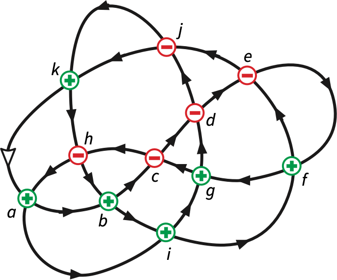
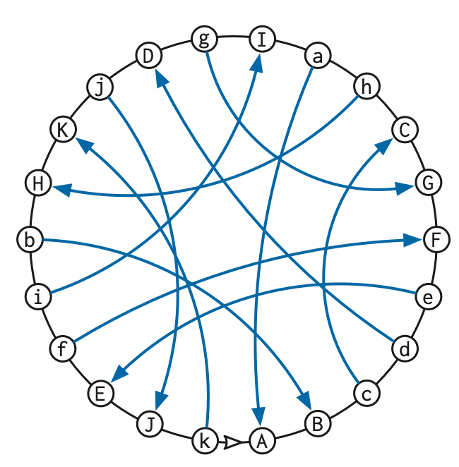
Assign a unique label to each vertex of the image graph of the curve. The Gauss code of a curve is the sequence of labels encountered by a point moving once around the curve, starting at an arbitrary basepoint and moving in an arbitrary direction. In other words, a Gauss code is a self-crossing sequence. Different choices of basepoint and direction lead to different Gauss codes. Specifically, changing the basepoint cyclically shifts the Gauss code, and changing direction reverses the Gauss code.
A signed Gauss code also records how the curve crosses itself at each vertex. Imagine a point moving along the curve in the chosen direction, starting at the chosen basepoint. The signed Gauss code records a positive crossing whenever the point crosses the curve from right to left, and a negative crossing whenever the point crosses the curve from left to right. (This is exactly the same sign convention that we used to compute winding number, from the point of view of the polygon.) Each vertex of the image graph of a curve appears twice in the curve’s signed Gauss code, once with each sign. I’ll typically indicate positive and negative crossings using upper- and lower-case letters, respectively. Again, different choices of basepoint and direction lead to different signed Gauss codes.
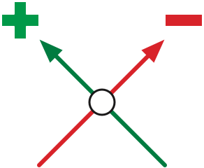
Figure 4 shows the curve from Figure 1, with a direction indicated by
arrows and a basepoint on the far left indicated by a white arrowhead.
Each vertex is labeled positive or negative according to the sign of the
first crossing through that vertex. The resulting signed Gauss
code is ABcdeFGChaIgDjKHbifEJK; by forgetting the signs, we
recover the unsigned Gauss code ABCDEFGCHAIGDJKHBIFEJK.
Gauss diagrams are an equivalent graphical representation of Gauss codes. A Gauss diagram for a curve with \(n\) self-intersections consists of an undirected cycle of \(2n\) nodes labeled by crossings, in the order they appear along the curve, along with edges joining the two appearances of each crossing point, directed from the negative crossing to the positive crossing. (Using directed edges here is slightly non-standard.)
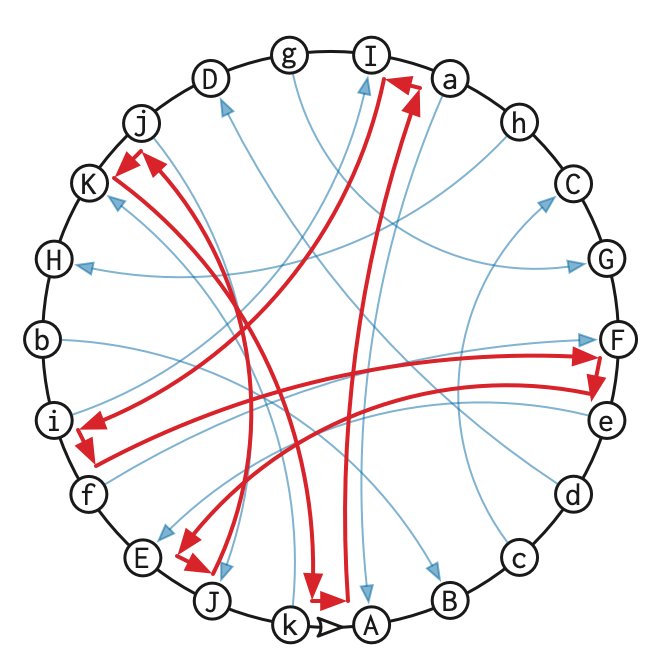
Perhaps surprisingly, we can completely recover the combinatorial structure of a curve from its signed Gauss code. I’ll justify this claim in more generality later, when we’ve built up more background on planar graphs, but we can already show one example, observed by Carter in the early 1990s [2]: The signed Gauss code implicitly encodes the faces of the curve.
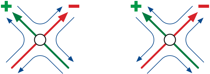
Imagine a point moving counterclockwise around the boundary of some face (or clockwise if the face is unbounded); the face always lies just to the left of the moving point. Between vertices, the point is either moving forward or backward along some edge of the image graph. At each crossing, the point turns to the left, as follows:
Similar case analysis allows us to trace a face to the right of a moving point, in clockwise order around the face, by turning right at every vertex.
(Pseudo)python (pseudo)code for Cater’s face-tracing algorithm is shown below. The first function computes the matching between different occurrences of the same crossing point; obviously this matching only needs to be extracted once if we want to trace several faces. With careful bookkeeping, we can extract all the faces of the curve directly from the signed Gauss code in \(O(n)\) time. Different Gauss codes for the same curve yield the same set of faces (but possibly with the vertices of each face rotated and/or reflected).
# extract matching between crossings from a signed Gauss code
#   input:  code = signed Gauss code
#           = permutation of list(range(-n,0)) + list(range(1,n+1))
#   output:  array match, defined by code[match[i]] = -code[i]
def indexCode(code):
    N = len(code)/2
    posindex = [0] * (N/2)
    match = [0} * N
    for i in range(N):
        if code[i] > 0:
            posindex[code[i] - 1] = i
    for i in range(N):
        if code[i] < 0:
            match[i] = posindex[1 - code[i]]
            match[match[i]] = i
    return match
# trace the face to the right of a moving point
# code = signed Gauss code (integers)
# start = index of starting edge (basepoint edge = 0)
# forward = boolean indicating starting direction
def traceFace(code, starti, forward):
match = matchCode(code)
N = len(code)
i = starti
while True:
next = forward ? i : (i + N - 1)%N
print(code[next])
if code[next] > 0:
forward = !forward
i = match[next]
if i = starti:
breakThe clockwise tracing process can be visualized on the Gauss diagram as follows. We start by tracing just inside an arc of the outer circle. Whenever we reach a crossing, we follow the interior edge across the diagram to its partner. If the crossing is positive, we stay on the same side of the interior edge; if the crossing is negative, we switch to the opposite side of the interior edge. Again, we can visualize counterclockwise tracing by a symmetric case analysis.
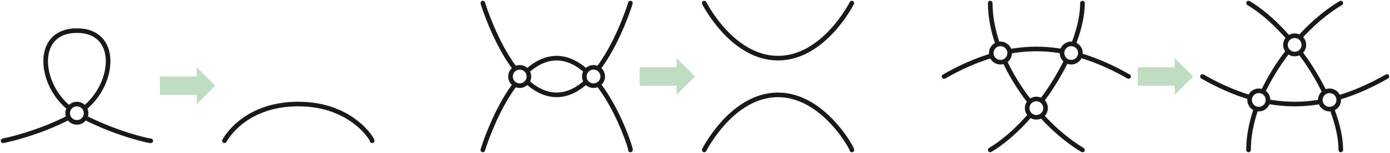
Every closed curve in the plane is homotopic to a point, and therefore to every other closed curve in the plane. However, it is still useful to study the structure of homotopies between generic curves. Recall that the simplicial approximation theorem let us approximate any homotopy between polygons as a finite sequence of vertex moves. If we make sufficiently small vertex moves that preserve genericity, each move incurs only a small local change in the pattern of self-intersections.
Careful case analysis implies that every homotopy between generic curves can be approximated by a finite sequence of homotopy moves of five different types. Each homotopy move modifies the curve only within a small neighborhood containing at most three vertices, leaving the rest of the curve unchanged outside this neighborhood.
In particular, we have the following:
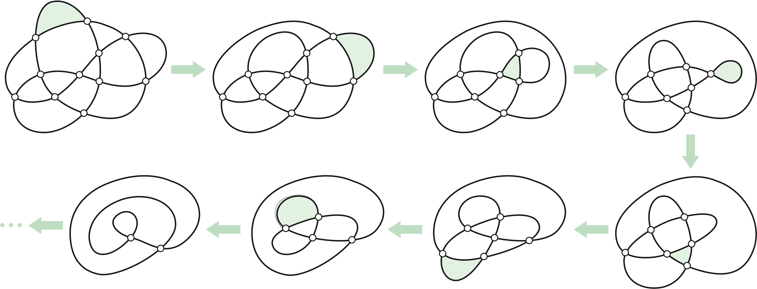
The proof of this theorem (via simplicial approximation) follows from the foundational work of Alexander and Briggs [1] and Reidemeister [2] on knot diagrams.3 This proof is fundamentally non-constructive; the number of homotopy moves we need depends on the geometric structure of the “given” homotopy. In a future lecture, we will see an algorithm, implicit in the work of Steinitz [3,4] a decade before Alexander, Briggs, or Reidemeister, that contracts any closed curve with \(n\) vertices using at most \(O(n^2)\) homotopy moves.
Each homotopy move can be implemented by locally modifying the Gauss code/diagram, or the equivalent data structures, as follows.
···Aa······Ab···Ba··· or
···aB···Ab······AB···bc···aC··· \(\mapsto\)
···BA···cb···Ca···.Every signed Gauss code is a signed double-permutation: A
string of even length, in which each symbol appears exactly twice, once
positive and once negative. However, not every signed double-permutation
is the signed Gauss code of a planar curve. For example, no planar curve
has the signed Gauss code ABab. (This is in fact the signed
Gauss code of a closed curve on the torus!) However, signed
Gauss codes of planar curves have a very simple characterization.
In all five cases, we have \(f-n = f'-n'\).
It follows by induction that if \(\gamma'\) is any curve reachable from \(\gamma\) by a finite sequence of homotopy moves, then \(f-n = f'-n'\). In particular, if \(\gamma'\) is simple, then \(n'=0\) and (by the Jordan curve theorem!) \(f'=2\), and therefore \(f-n = 2\).
In fact, the converse of this lemma is also true, although we don’t yet have the tools to prove it:
If you have played with played with planar graphs before, you might recognize this theorem as an avatar of Euler’s formula \(V-E+F = 2\). Because every vertex in the image graph of any non-simple curve has degree \(4\), the number of edges is exactly twice the number of vertices.
James W. Alexander and Garland B. Briggs. On types of knotted curves. Ann. Math. 28(1/4):562–586, 1926–1927. Reidemeister moves, with pictures.
J. Scott Carter. Classifying immersed curves. Proc. Amer. Math. Soc. 111(1):281–287, 1991. The face-tracing algorithm to reconstruct curves from signed Gauss codes.
Kurt Reidemeister. Elementare Begründung der Knotentheorie. Abh. Math. Sem. Hamburg 5:24–32, 1927. Reidemeister moves, without pictures.
Ernst Steinitz. Polyeder und Raumeinteilungen. Enzyklopädie der mathematischen Wissenschaften mit Einschluss ihrer Anwendungen III.AB(12):1–139, 1916. Proof of “Steinitz’s theorem” — Every 3-connected planar graph is the 1-skeleton of a convex polyhedron — using \(3\mathord\to 3\) homotopy moves in the medial graph. I promise those words will eventually make sense.
Ernst Steinitz and Hans Rademacher. Vorlesungen über die Theorie der Polyeder: unter Einschluß der Elemente der Topologie. Grundlehren der mathematischen Wissenschaften 41. Springer-Verlag, 1934. Reprinted 1976. More detailed proof of “Steinitz’s theorem”, with pictures.
Consider shuffling the topics in lectures 6–8:
We’re admittedly getting a little ahead of ourselves here. A plane graph is any graph whose vertices are points in the plane, and whose edges are interior-disjoint paths between their endpoints.↩︎
Stop trying to make “digon” and “trigon” happen, Gretchen. They’re not going to happen.↩︎
A knot diagram is generic closed curve with additional data at each crossing, indicating which branch of the curve passes in front of the other. Homotopy moves that sensibly preserves this crossing data are called Reidemeister moves.↩︎