In the last lecture, we saw a simple algorithm to test whether a signed Gauss code is consistent with a generic curve in the plane: Count the faces (by symbol-chasing) and return true if and only if the number of faces is exactly two more than the number of crossings.
In his unpublished notes, written around 1840, Gauss was asked how to determine whether an unsigned Gauss code is consistent with a planar curve [3]. The same question was published about 40 years later by Tait [8]. I regard this as the first problem in computational topology. (Euler’s famous Bridges of Königsberg is the zeroth problem in computational topology.) B oht Gauss and Tait described a partial solution to his problem. The first complete solution was proposed by Julius Nagy almost a century later [4].1
In this lecture, I’ll describe an \(O(n^2)\)-time algorithm originally described by Max Dehn in 1936 [1], with some simplifications suggested by Nagy’s solution and more modern graph algorithms, as suggested by Read and Rosenstiehl [11], Rosenstiehl and Tarjan [12], and de Fraysseix and Ossona de Mendez [3].2 My presentation of Dehn’s algorithm also closely follows Kaufmann. [[Fix reference numbers]]
Recall that the winding number of a polygon \(P\) around a point \(o\) can be computed by shooting a vertical ray from \(o\) and counting positive and negative crossings with the polygon. The same characterization extends to generic curves, but it’s a little unsatisfying, for a couple of reasons. First, we only care about curves up to isotopy, but the ray-shooting algorithm requires choosing a specific (arbitrary) curve in the isotopy class. We can soften this objection somewhat by observing that we don’t really need to count crossings with a ray; any path from \(o\) to infinity that crosses the curve a finite number of times will work.
But there’s a more serious objection. Our representation of closed curves (signed Gauss codes) doesn’t include any geometric information. But how do we represent the point? We can’t give coordinates, because different curves with the same representation have different winding numbers around any fixed point!
Instead, we specify the obstacle point \(o\) by declaring which face of the curve contains it. More cleanly, we define the winding number of a curve \(\gamma\) around each of its faces using an Alexander numbering, we defined in Lecture 2 for polygons. For any directed edge \(e\) of the image graph, let \(\textsf{left}(e)\) and \(\textsf{right}(e)\) denote the faces immediately to the left and right of \(e\) (relative to the orientation of \(e\)).
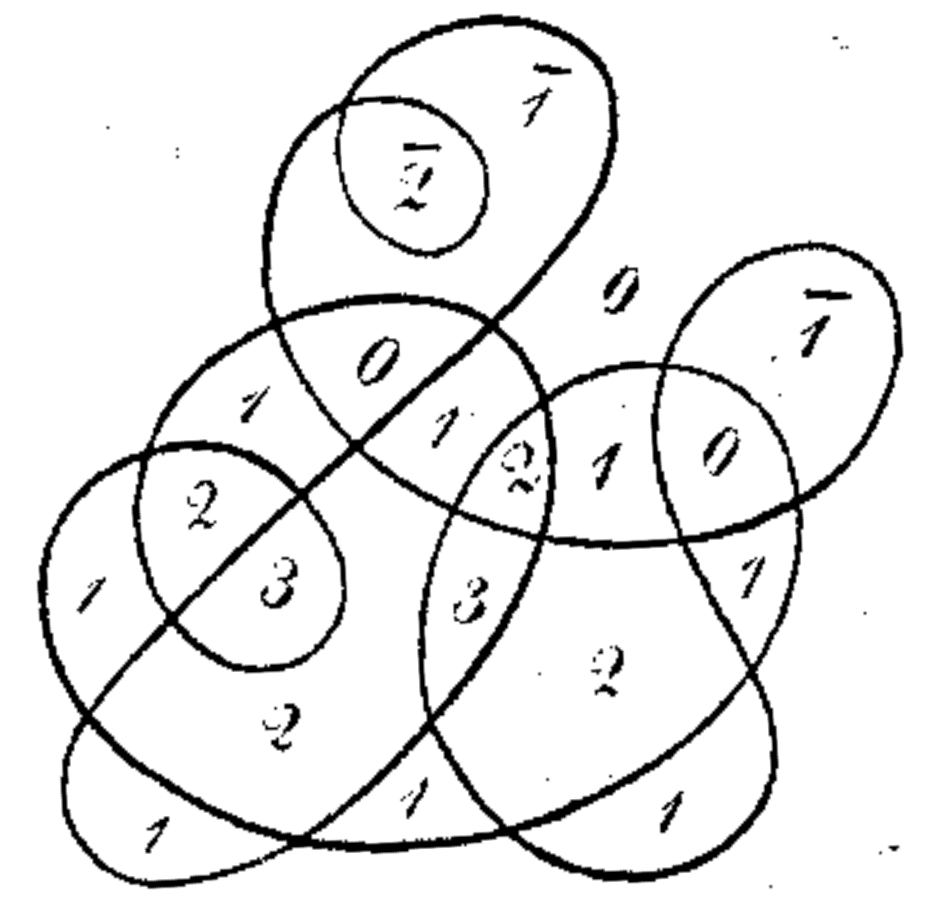
Gauss observed that we can also define winding numbers by smoothing the curve at each vertex. Smoothing replaces a neighborhood of a single vertex with a pair of disjoint curve segments. In fact there are two different smoothing operations, depending on how the disjoint curve segments are attached. One smoothing operation disconnects the curve (or connects two constituents of a multicurve) but preserves the direction of both subcurves. The other keeps the curve connected, but requires the direction of part of the curve to be reversed.
Gauss observed that by smoothing every vertex of a curve to preserve direction, we can decompose the curve into a finite set of disjoint simple curves. This collection of simple curves is called the Seifert decomposition of the curve. Each of these simple curves has winding number \(+1\) or \(-1\) around its interior, depending whether the curve is oriented counterclockwise or clockwise.
The winding number of a curve \(\gamma\) around any point \(o\) (far from the vertices) is equal to the sum of the winding numbers of the curves in the Seifert decomposition of \(\gamma\) around \(o\). Equivalently, \(\textsf{wind}(\gamma, 0)\) is equal to the number of counterclockwise cycles that contain \(o\) minus the number of clockwise cycles that contain \(o\).
Gauss observed without proof that the unsigned Gauss code of every planar curve satisfies a simple parity condition: Every substring that starts and ends with the same symbol has even length, or equivalently, each symbol appears once at an even index and once at an odd index. This parity condition was first proved necessary by Nagy. The following simpler combinatorial proof is due to Rademacher and Toeplitz.
Now let \(X\) be a string of length 2n, in which each of the \(n\) unique symbols appears twice.
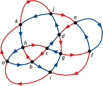
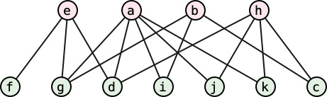
We can test this parity condition in \(O(n^2)\) time by brute force, but in fact, there is a simple linear-time algorithm. Given the Gauss code \(X\), we can define a directed graph \(G(X)\), which I’ll call the Nagy graph of \(X\), as follows:
abcdefgchaigdjkhbifejk contains the following edges:
\[
a\mathord\rightarrow b\mathord\leftarrow
c\mathord\rightarrow d\mathord\leftarrow
e\mathord\rightarrow f\mathord\leftarrow
g\mathord\rightarrow c\mathord\leftarrow
h\mathord\rightarrow a\mathord\leftarrow
i\mathord\rightarrow g\mathord\leftarrow
d\mathord\rightarrow j\mathord\leftarrow
k\mathord\rightarrow h\mathord\leftarrow
b\mathord\rightarrow i\mathord\leftarrow
f\mathord\rightarrow e\mathord\leftarrow
j\mathord\rightarrow k\mathord\leftarrow a
\]Let me emphasize (despite the figure below) that the Nagy graph of a string is an abstract graph, which may or may not be planar.
Now imagine a point moving around the Nagy graph \(G(X)\), alternately traversing edges forward and backward in the order they appear in \(X\). Whenever the point passes through a vertex of \(G(X)\), it either traverses two inward edges \(u\mathord\rightarrow v\mathord\leftarrow w\) (one forward and one backward) or two outward edges \(u\mathord\leftarrow v\mathord\rightarrow w\) (one backward and one forward). The parity condition implies that if we leave any vertex \(v\) along a forward edge \(v\mathord\to w\), we will next enter \(v\) along a backward edge \(x\mathord\leftarrow v\) and v vice versa. In fact, these two conditions are equivalent.
If a Gauss code does not satisfy the parity condition, then its Nagy graph will contain at least one vertex with in-degree 0 and out-degree 4, and an equal number of vertices with in-degree \(4\) and out-degree \(0\).
We can easily construct the Nagy graph and check the degree of each vertex in \(O(n)\) time, where \(X\) is the length of the given Gauss code. (There are simpler algorithms to check the parity condition in \(O(n)\) time, but we’ll need the Nagy graph later, so we might as well build it now.)
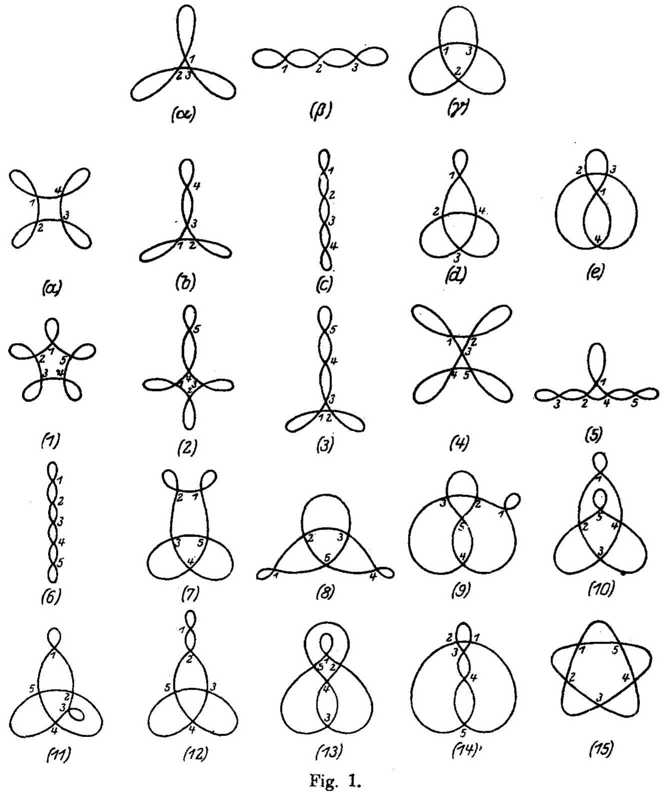
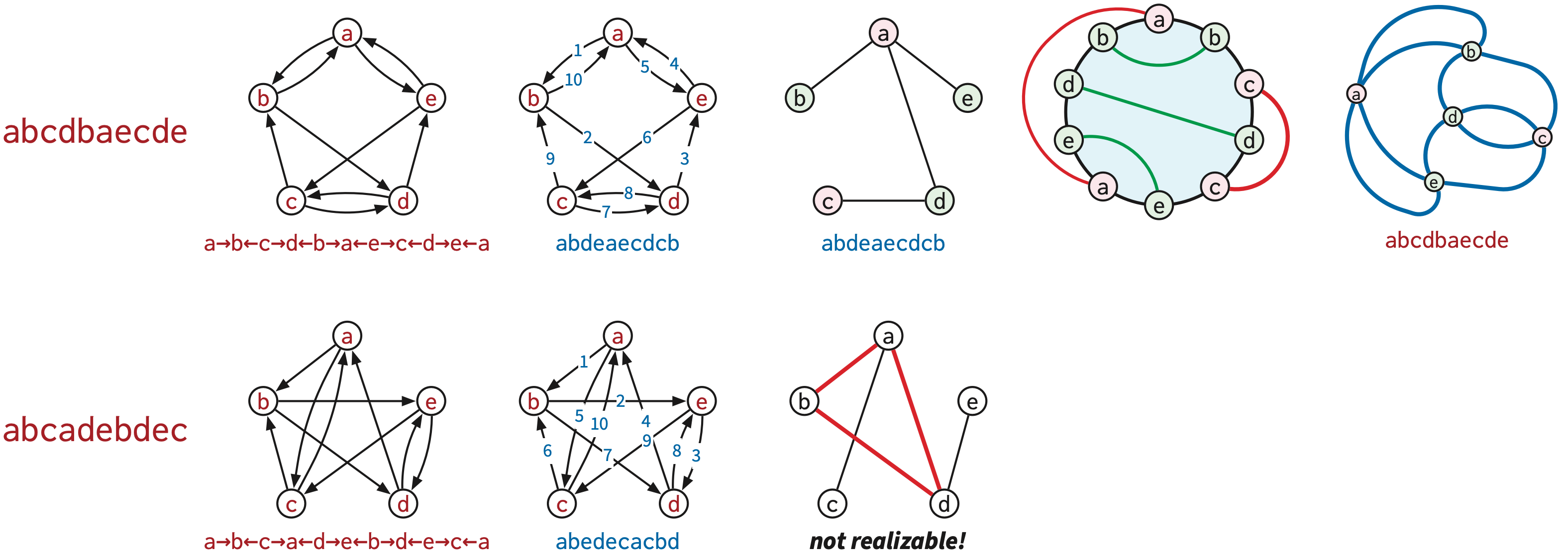
Gauss also observed that the sequences abcadcedbe and
abcabdecde satisfy his parity condition but cannot be
realized by planar curves, so the parity condition is not sufficient.
Tait later gave a third example abcadebdec.
About 100 years after Gauss, Dehn [1] described das Gaussische Problem der Trakte and proposed an algorithm to solve it. Dehn observed that smoothing every vertex of a curve to keep the curve connected results in a simple closed curve that touches itself at every vertex. The same closed curve \(\gamma\) can have several different connected smoothings.
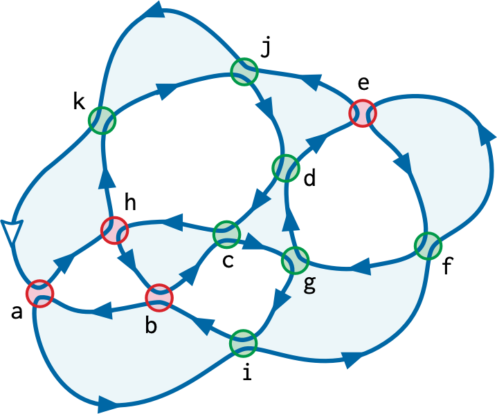
On the other hand, the edges incident to any vertex of \(G(X(\gamma))\) alternative in, out, in, out in cyclic order. Thus, every Euler tour of \(G(X(\gamma))\) touches itself at every vertex, but never crosses itself. It follows that every Euler tour of \(G(X(\gamma))\) is a connected smoothing of \(\gamma\).
On the other hand, suppose \(G(X)\) has a planar embedding with a weakly simple Euler tour. Then the edges incident to each vertex in that embedding must alternate in-out-in-out in cyclic order. The original Gauss code \(X\) defines an undirected Euler tour \(U\) of \(G(X)\), which traverses edges of \(G(X)\) alternately forward and backward. \(U\) crosses itself at every vertex of \(G(X)\). It follows immediately that \(U\) is a closed curve with Gauss code \(X\).
Dehn described a symbolic algorithm to test his non-crossing condition in terms of the sequence of self-touching points in order along the smoothed curve \(\tilde\gamma\). Just like Gauss codes, this sequence contains exactly two occurrences of every symbol. To distinguish this sequence from the Gauss code of a curve, I’ll refer to this new string as a Dehn code. We can similarly define the Dehn diagram of \(\tilde\gamma\) as a cycle of \(2n\) vertices, corresponding to the labels in the Dehn code, plus chords connecting identical labels.3
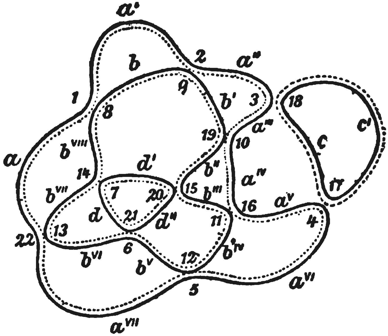
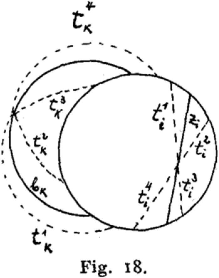
Dehn observed that the Dehn diagram of any connected smoothing \(\tilde\gamma\) of any planar curve \(\gamma\) is a planar graph; that is, we can embed some of the chords of the diagram inside the circle and the rest outside the circle, so that no pair of chords intersects. Specifically, if we perturb \(\tilde\gamma\) slightly into a simple curve, the neighborhood of each vertex either has connected intersection with the interior of \(\tilde\gamma\) or connected intersection with the exterior of \(\tilde\gamma\). These vertices correspond to inner and outer chords, respectively.
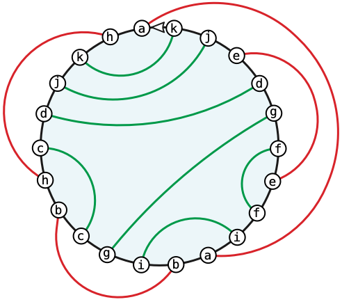
Dehn playfully referred to these planar diagrams as “Baum-Zwiebel Figuren” [“tree-onion diagrams”] and their corresponding Gauss codes as “Baum-Zwiebel Reihen” [“tree-onion strings”]. Tree onions, also known as walking onions or Egyptian onions, are onion cultivars that grow clusters of small bulbs at the top of the stem, where other Allium species have flowers. The chords of a tree-onion figure (loosely) resemble clusters of onion layers. Coincidentally(?), the dual graph of the inner chords (or the outer chords) of any tree-onion figure is a tree.4
![A tree-onion figure [Dehn 1936]](Fig/Dehn-BZ-Figur.png)
![Tree onion bulblets. [Kurt Stüber 2004, CC BY-SA 3.0, via Wikimedia Commons]](Fig/tree-onion-photo.jpg)

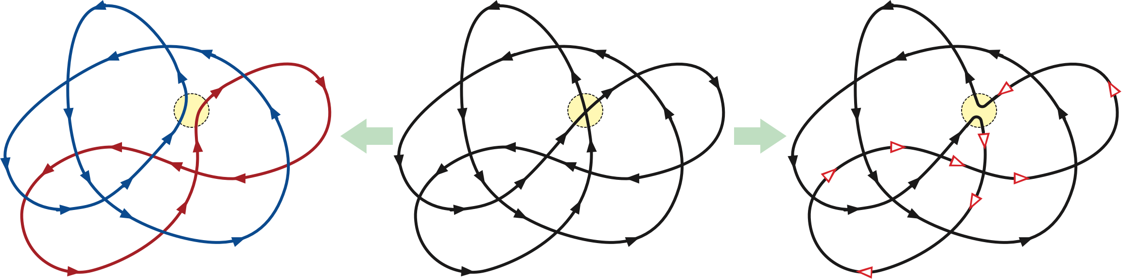
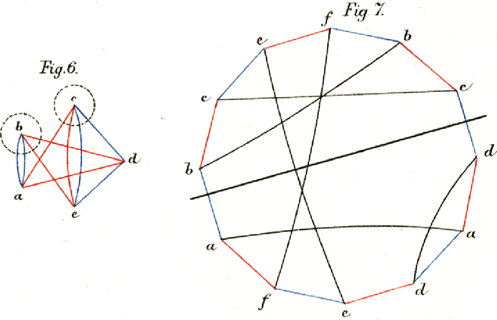
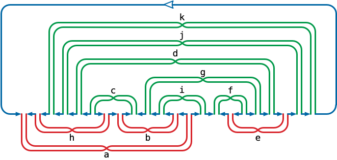
(Petersen [9] used similar diagrams in 1891 to study abstract regular graphs. Consider a connected \(4\)-regular graph \(G\) with \(n\) vertices. Petersen defined a “stretched graph” by representing any Euler tour of \(G\) as a cycle of length \(2n\), with additional edges connecting the two occurrence of each vertex of \(G\). If we alternately color the edges this cycle red and blue, every vertex of \(G\) is incident to two edges of each color. Thus, every \(4\)-regular graph can be decomposed into two 2-factors. Applying Petersen’s construction to any curve, as an Euler tour of its image graph, recovers the forward and backward cycles in the curve’s Nagy graph.)
Read and Rosenstiehl [6] observed that Dehn’s planarity condition can verified efficiently by constructing yet another graph, called the interlacement graph of the Dehn code. The interlacement graph has \(n\) vertices, one for each symbol, and an edge between any two symbols \(x\) and \(y\) whose appearances are interlaced \(x\dots y \dots x\dots y\) in the Dehn code. Partitioning the chords of a Dehn diagram into pairwise disjoint inner and outer chords is equivalent to partitioning the vertices of the interlacement graph into two independent sets. In other words, a Dehn diagram is planar if and only if its interlacement graph is bipartite.
To complete his algorithm, Dehn observed that we can transform the Dehn diagram of any Euler tour of \(G(X)\) into a 4-regular graph by replacing each chord with a pair of crossing chords with a crossing, as shown below. Assuming the interlacement graph of the Dehn code is bipartite, the corresponding Dehn diagram is planar, so this recrossing process yields a single closed curve consistent with our original Gauss code \(X\).
Putting all the pieces together, we conclude:
There are several linear-time algorithms to test the interlacement condition without explicitly constructing the interlacement graph, but we’re out of time.
Max Dehn. Über kombinatorishe Topologie. Acta Math. 67:123–168, 1936.
Clifford H. Dowker and Morwen B. Thistlethwaite. Classification of knot projections. Topology Appl. 16(1):19–31, 1983.
Hubert de Fraysseix and Patrice Ossona de Mendez. A short proof of a Gauss problem. Proc. 5th Int. Symp. Graph Drawing, 230–235, 1997. Lecture Notes Comput. Sci. 1353, Springer.
Carl Friedrich Gauß. Nachlass. I. Zur Geometria situs. Werke, vol. 8, 271–281, 1900. Teubner. Originally written between 1823 and 1840.
Carl Hierholzer. Über die Möglichkeit, einen Linienzug Ohne Wiederholung und ohne Unterbrech nung zu umfahren. Math. Ann. 6:30–32, 1873.
Louis H. Kauffman. Gauss codes, quantum groups and ribbon Hopf algebras. Rev. Math, Phys. 5(4):735–773, 1993.
Louis H. Kauffman. Virtual knot theory. Europ. J. Combin. 20(7):663–691, 1999. arXiv:math/9811028.
Julius v. Sz. Nagy. Über ein topologisches Problem von Gauß. Math. Z. 26(1):579–592, 1927.
Julius Petersen. Die Theorie der regulären graphs. Acta Math. 15:193–220, 1891. Yes, really, “graphs” not “Graphen”.
Hans Rademacher and Otto Toeplitz. On closed self-intersecting curves. The Enjoyment of Mathematics: Selections from Mathematics for the Amateur, chapter 10, 61–66, 1990. Dover Publ. Originally published by Princeton Univ. Press, 1957.
Ronald C. Read and Pierre Rosenstiehl. On the Gauss crossing problem. Combinatorics, 843–876, 1976. Colloq. Math. Soc. János Bolyai 18, North-Holland. Modern description of Dehn’s solution to the Gauss code problem.
Pierre Rosenstiehl and Robert E. Tarjan. Gauss codes, planar Hamiltonian graphs, and stack-sortable permutations. J. Algorithms 5(3):375–390, 1984. Linear-time implementation of Dehn’s solution to the Gauss code problem.
Peter Guthrie Tait. On knots I. Trans. Royal Soc. Edinburgh 28(1):145–190, 1876–7.
Nagy’s algorithm attempts to construct a Seifert decomposition of the encoded curve. I’m afraid I don’t understand Nagy’s solution well enough to describe it, or even to be confident that it is correct.↩︎
Dozens of other combinatorial and algebraic characterizations of planar Gauss codes have been published since Dehn’s solution, but as far as I know, none lead to a simpler or more efficient algorithm (except through the use of linear-time algorithms to test graph planarity, which is cheating).↩︎
The terms “Dehn code” and “Dehn diagram” are nonstandard.↩︎
Tree-onion figures are also closely related to tree-cotree decompositions of planar maps. Specifically, there is a bijection between tree-cotree decompositions of a planar map \(\Sigma\) and tree-onion figures of non-crossing Euler tours of the medial map \(\Sigma^\times\). (Don’t worry; those words will make sense soon.) So it’s really tempting to refer to the partition of inner and outer chords in a tree-onion figure as a coonion-onion decomposition.↩︎