We need to establish definitions for a few important structures in graphs. Most of these are likely already familiar; I recommend using this list as later reference rather than reading it as text. Move to end of previous note?
Let’s begin by discussing two operations for modifying abstract graphs. Let \(G\) be an arbitrary connected (but not necessarily planar) abstract graph with \(n\) vertices and \(m\) edges.
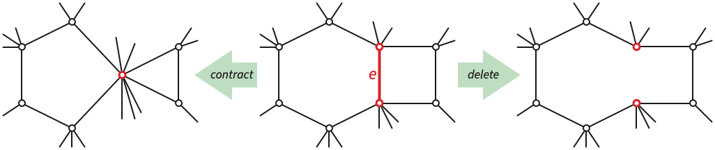
Deleting an edge \(e\) from G yields a smaller graph \(G \setminus e\) with \(n\) vertices and \(m-1\) edges. We also write \(G \setminus v\) to denote the graph obtained from \(G\) by deleting a vertex \(v\) and all its incident edges. Deleting a bridge disconnects the graph.
Symmetrically, if \(e\) is not a loop, then contracting \(e\) merges the endpoints of \(e\) into a single vertex and destroys the edge, yielding a smaller graph \(G \mathbin/ e\) with \(n - 1\) vertices and \(m-1\) edges. Contracting a loop is simply forbidden by definition. Contracting a loop is not (yet) defined. If \(G\) contains edges parallel to \(e\), those edges survive in \(G \mathbin/ e\) as loops.
A subgraph of a graph \(G\) is another graph obtained from \(G\) by deleting edges and isolated vertices; a proper subgraph of \(G\) is any subgraph other than \(G\) itself. (We often equate subgraphs of \(G\) with subsets of the edges of \(G\).) Deleting any subset of edges \(E’ \subseteq E\) that does not contain a bond yields a connected proper subgraph \(G \setminus E’\).
Symmetrically, contracting any subset of edges \(E’ \subseteq E\) that does not contain a cycle yields a proper minor \(G \mathbin/ E’\). A minor of \(G\) is any graph obtained from a subgraph of \(G\) by contracting edges; a proper minor of \(G\) is any minor other than \(G\) itself.
The inverse of deletion is called insertion, and the inverse of contraction is called expansion. If \(G\) is a (proper) subgraph of another graph \(H\), then \(H\) is a (proper) supergraph of \(G\); similarly, if \(G\) is a (proper) minor of \(H\), then \(H\) is a (proper) major of \(G\).
A spanning tree of a graph \(G\) is a connected, acyclic subgraph of \(G\) (more more succinctly, a subtree of \(G\)) that includes every vertex of \(G\). We leave the following lemma as an exercise for the reader.
This lemma immediately suggests the following general strategy to compute a spanning tree of any connected graph: For each edge \(e\), either contract \(e\) or delete \(e\). Loops must be deleted and bridges must be contracted; otherwise, the decision to contract or delete is arbitrary. (It is impossible for an edge to be both a bridge and a loop!) The previous lemma implies by induction that the set of contracted edges is a spanning tree of \(G\), regardless of the order that edges are visited, or which non-loop non-bridge edges are deleted or contracted.
In practice, algorithms that compute spanning trees do not actually contract or delete edges; rather, they simply label the edges as either belonging to the spanning tree or not. In this context, the previous lemma can be rewritten as follows:
Given a connected graph with \(n\) vertices and \(m\) edges, we can compute a spanning tree in \(O(n+m)\) time using any number of graph traversal algorithms, the most common of which are depth-first search and breadth-first search. These algorithms can be seen as variants of the red-blue coloring algorithm, where the order in which edges are colored (or equivalently, the choice of edges to delete or contract) is determined on the fly as the algorithm explores the graph.
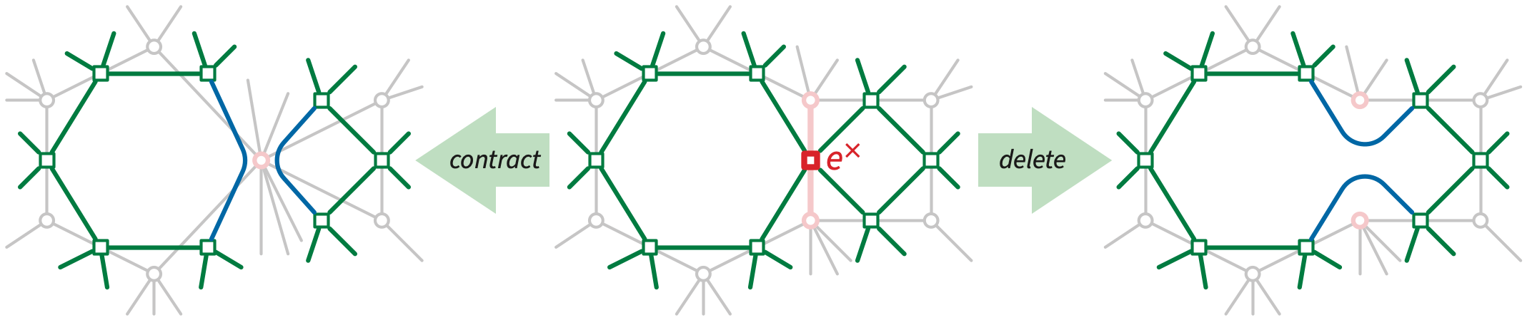
Contraction and deletion play complementary roles in planar maps. For example, contracting any (non-loop) edge identifies its two endpoints; deleting any (non-bridge) edge merges its two shores. This resemblance is not merely incidental; in fact, contraction and deletion are dual operations. Contracting an edge in any map \(\Sigma\) is equivalent to deleting the corresponding edge in \(\Sigma^*\) and vice versa.
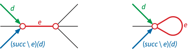
Hopefully this duality is intuitively clear, but we can make it formally trivial by describing how deletion and contraction are implemented in planar maps. Let \(\textsf{succ}\) denote the successor permutation of a planar map \(\Sigma\), and let \(\textsf{succ}^* = \textsf{rev}\circ \textsf{succ}\) denote its dual successor permutation, which is also the successor permutation of the dual map \(\Sigma^*\). Fix an arbitrary edge \(e\) of \(\Sigma\).
It follows that the dual successor permutation changes as follows: \[ (\textsf{succ}^*\setminus e)(d) = \begin{cases} \textsf{succ}^*(\textsf{succ}(\textsf{succ}(d))) & \text{if $\textsf{succ}(d) \in e$ and $\textsf{succ}(\textsf{succ}(d)) \in e$,}\\ \textsf{succ}^*(\textsf{succ}(d)) & \text{if $\textsf{succ}(d) \in e$,}\\ \textsf{succ}^*(d) & \text{otherwise.} \end{cases} \]
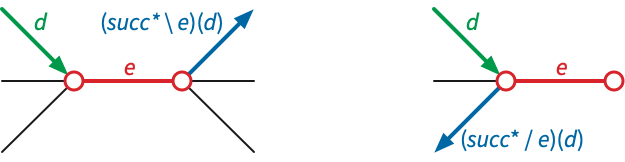
It follows that the primal successor permutation changes as follows: \[ (\textsf{succ} \mathbin/ e)(d) = \begin{cases} \textsf{succ}(\textsf{succ}^*(\textsf{succ}^*(d))) & \text{if $\textsf{succ}(d) \in e$ and $\textsf{succ}^*(\textsf{succ}^*(d)) \in e$,}\\ \textsf{succ}(\textsf{succ}^*(d)) & \text{if $\textsf{succ}(d) \in e$,}\\ \textsf{succ}(d) & \text{otherwise.} \end{cases} \]
Both of these formulas are trivially correct when we either delete or contract the only edge in a one-edge map, because the resulting trivial map has no darts. Assuming standard data structures, any edge can be contracted or deleted in \(O(1)\) time.
The following lemma is now purely mechanical.
If we delete a bridge using the formulas above, the components of \(G\setminus e\) become embedded independently, each on its own plane/sphere; instead of merging two faces into one, the deletion breaks one face (on either side of the deleted edge) into two. Symmetrically, if we contract a loop using the formula above, instead of merging two vertices into one, we split the single endpoint of the loop into two, splitting the graph into two independent subgraphs, one “inside” the loop and the other “outside”.
On the other hand, let \(H^*\) is an edge cut in \(\Sigma^*\). Then it is possible to color the vertices of \(\Sigma^*\) black and white, so that \(H^*\) is the subset of edges with one white endpoint and one black endpoint. The primal subgraph \(H\) contains precisely the edges of \(\Sigma\) with one white shore and one black shore. Every vertex of \(\Sigma\) is incident to an even number of such edges. We conclude that \(H\) is an even subgraph of \(\Sigma\).
Equivalently, a cycle is a minimal subset of edges that cannot all be contracted, and a bond is a minimal subset of edges that cannot all be deleted.
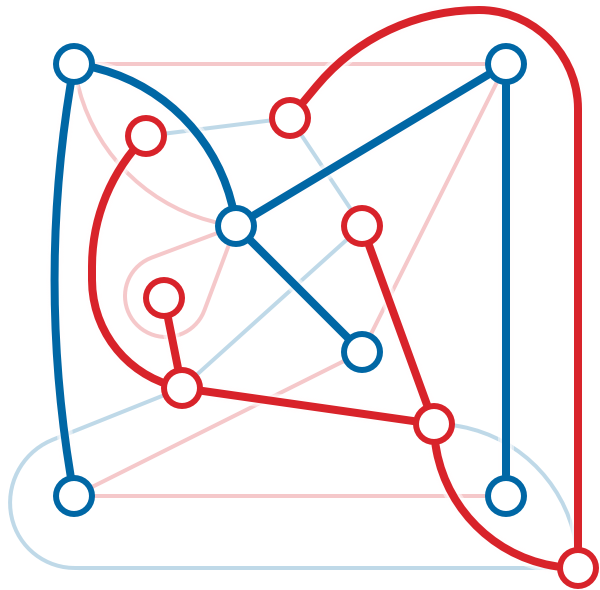
The partition \(T\sqcup C\) of edges of a planar map into primal and dual spanning trees is called a tree-cotree decomposition. Notice that either the primal spanning tree \(T\) or the dual spanning tree \(C^*\) can be chosen arbitrarily.
The duality between cycles and bonds was first proved by Hassler Whitney. Whitney also proved the following converse result. An algebraic dual of an abstract graph \(G\) is another abstract graph \(G^*\) with the same set of edges, such that a subset of edges defines a cycle in \(G\) if and only if the same subset defines a bond in \(G^*\).
Theorem (Whitney (1932)): A connected abstract graph is planar if and only if it has an algebraic dual.
Arguably the earliest fundamental result in combinatorial topology is a simple formula first published by Leonhard Euler, but described in full generality over a century earlier by René Descartes, and described for the special case of Platonic solids by Francesco Maurolico a century before Descartes. I’ll provide two short proofs here, one directly inductive, the other relying on tree-cotree decompositions.
In all cases, we conclude that \(n-m+f=2\).
There are many many other proofs of Euler’s formula. David Eppstein has a web page describing more than twenty of them, but even David’s list is incomplete. For example, we can leverage our earlier proof of Euler’s formula for planar curves, after establishing a few additional definitions.
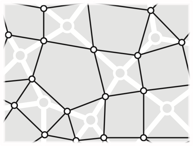
Recall that the medial map \(\Sigma^\times\) of a planar map \(\Sigma\) is another planar map whose vertices correspond to edges of \(\Sigma\), whose edges correspond to corners of \(\Sigma\), and whose faces correspond to vertices and faces of \(\Sigma\). Every medial map \(\Sigma^\times\) is either a simple cycle or 4-regular, and therefore is the image map of a connected planar multicurve. (Steinitz used medial maps (“\(\Theta\)-Prozeß”) to reduce his eponymous theorem about graphs of convex polyhedra to an argument about curves.)
I’ll close this lecture by proving a powerful reformulation of Euler’s formula.
Suppose we assign a value \(\angle c\) to each corner \(c\) of a planar map \(\Sigma\), called the exterior angle at \(c\). Intuitively, you should think of \(\angle c\) as the signed angle between the tangent vectors to two darts \(d\) and \(\textsf{succ}^*(d)\) at their common endpoint \(\textsf{head}(d)\), but in fact \(\angle c\) can be any real (or complex!) number. As usual, we measure angles in units of circles (or “turns”), as the gods intended.
We can then define the combinatorial curvature of a face \(f\) or a vertex \(v\), with respect to this angle assignment, as follows: \[ \kappa(f) := 1 - \sum_{c\in f} \angle c \qquad\qquad \kappa(v) := 1 - \frac{1}{2} \deg(v) + \sum_{c\in v} \angle c \] Or more formally, equating corners with darts: \[ \kappa(f) := 1 - \sum_{d \colon \textsf{left}(d) = f} \angle d \qquad\qquad \kappa(v) := 1 - \sum_{d \colon \textsf{head}(d) = v} \left(\frac12 - \angle d\right) \]
For example, suppose every edge of \(\Sigma\) is a line segment, and we actually measure corner angles geometrically. Then every vertex has curvature \(0\) (because its interior corner angles sum to one circle) and every bounded face of \(\Sigma\) has curvature \(0\) (because its total turning angle is \(1\)). However, the the outer face is oriented clockwise instead of counterclockwise, so its total turning angle is \(-1\), and thus its curvature is \(2\). That \(2\) is actually the same as the \(2\) in Euler’s formula.
Alternatively, suppose \(\Sigma\) is actually embedded on the unit sphere, every edge is an arc of a great circle, and angles are again measured geometrically (between tangent vectors). Then every vertex of \(\Sigma\) has curvature zero, because interior angles at any vertex sum to one circle, and a bit of spherical trigonometry implies that every face of \(\Sigma\) has curvature equal to its area divided by \(2\pi\). Because the unit sphere has surface area \(4\pi\), the sum of all the face curvatures is \(2\). That \(2\) is actually the same as the \(2\) in Euler’s formula! (In fact, this is how Lagrange actually proved Euler’s formula for the first time.)
As a final geometric example, suppose \(\Sigma\) is actually the complex of vertices, edges, and faces of a three-dimensional convex polyhedron (which is homeomorphic to a sphere), and again, angles are measured geometrically. Each face of \(\Sigma\) is a convex planar polygon, and therefore has curvature zero. The interior angles at each vertex of \(\Sigma\) sum to less than a full circle, so every vertex has positive curvature. The Combinatorial Gauss-Bonnet Theorem implies that the sum of the vertex curvatures is exactly \(2\). In other words, the sum of the angle defects at the vertices is two full circles, or eight right angles.
Euler’s formula has a long and convoluted history, involving unpublished and lost manuscripts, quack medicine, boat wrecks, priority battles, bad translations, incorrect proofs, and philosophical arguments over the natural of mathematical proof. At the risk of adding to the thousands of gallons of ink, seat, and blood that have already been spilled over this history, let me briefly mention a few highlights.
The first known statement of Euler’s formula is in an unpublished manuscript Compaginationes solidorum regularium (Combinations of regular solids) written by Francesco Maurolico between 1536 and 1537.
Item manifestum est in unoquoque regularium solidorum, numerum basium coniunctum cum numero cacuminum conflare numerum, qui binario excedit numerum laterum. [It is obvious that in each of the regular solids, the number of bases (faces) combined with the number of peaks (vertices) is a number that exceeds the number of sides (edges) by 2.]
Maurolico only considered the five Platonic solids, for which the formula follows by direct inspection.
René Descartes described the angle defect theorem for convex polyhedra, and derived Euler’s formula from it, in his unpublished note Progymnasmata de solidorum elementis [Exercises in the Elements of Solids], written around 1630.
Ponam semper pro numero angulorum solidorum \(\alpha\) & pro numero facirum \(\varphi\dots\). Numerus verorum angulorum planorum est \(2\varphi - 2\alpha - 4\). [I always write \(\alpha\) for the number of solid angles (vertices) and \(\varphi\) for the number of faces\(\dots\). The total number of plane angles (corners) is \(2\varphi - 2\alpha - 4\).]
It is a matter of surprisingly intense scholarly dispute whether Descartes actually stated Euler’s formula, and therefore deserves to share credit with Euler, or only came close, and therefore does not. Descartes did not express his formula using the syntax \(V-E+F=2\), but in my opinion, this is entirely a matter of notational emphasis, not content or understanding. Elsewhere in Progymnasmata, Descartes observed that the number of plane angles is exactly twice the number of edges, and he used the numbers of vertices, edges, and faces of the Platonic and several Archimedean solids to derive formulas for corresponding figurate numbers. Had Descartes actually published his Progymnasmata, I believe even Euler (who exhibited surprise that the formula was not already known) would have called it “Descartes’ formula”.
Descartes traveled to Sweden in 1649 at the invitation of then-19-year-old Queen Christina. Due to his poor health, Descartes normally slept late, but after a few months, the young queen required Descartes to give her lessons in philosophy three days a week, lasting five hours per day and beginning at 5am. Within a month, Descartes fell ill. He refused the treatments offered by the Swedish doctors, preferring his own French doctor’s prescription of tobacco-infused wine to induce vomiting. The treatment proved ineffective, and Descartes eventually died of pneumonia in February 1650.
After Descartes’ death, his possessions were shipped to his friend Claude Clerselier in Paris; upon arrival, a box of manuscripts, including the Progymnasmata, fell into the Seine and was not recovered for three days. Clerselier rescued Descartes’ manuscripts, and after carefully drying them, made them available to other scholars.
Gottfried Leibniz transcribed several of Descartes’ manuscripts, including the Progymnasmata, during a trip to Paris in 1676, most likely in an effort to collect evidence against recent charges by English mathematicians that his results were merely elaborations of Descartes’ ideas. (Isaac Newton charged Leibniz of plagiarizing his calculus later that same year.) Descartes’ original manuscript was then lost forever. Leibniz’s hand-written copy vanished into his archives until 1859, when it was rediscovered by Louis Alexandre Foucher de Careil in an uncatalogued pile of Leibniz’s papers.2 Foucher de Careil published Leibniz’s transcription , but his re-transcription introduced several significant errors, rendering it essentially useless. An accurate transcription of the finally appeared in 1908.
Leonhard Euler stated both his eponymous formula and the angle defect theorem for convex polyhedra, expressing surprise that neither was previously known, in a letter to his friend and colleague Christian Goldbach in 1750. Two years later, he proposed an inductive proof to the St. Petersberg Academy of Sciences; unfortunately his proof was flawed. Similarly flawed inductive proofs were published by Karsten in 1768, by Meister in 1785, by L’Huillier in 1811, by Cauchy in 1813, and by Grunert in 1827. One of Cauchy’s inductive arguments is presented in numerous textbooks as the first correct proof of Euler’s formula, but that claim is incorrect for at least three reasons: The argument is not original to Cauchy; the argument is not a proof; and a correct proof was already known.3
Cauchy argued as follows: Consider a simple planar map \(\Sigma\) whose bounded faces are all triangles and whose outer face is a simple cycle. Let \(f\) be any face that has at least one edge on the outer face. If \(f\) shares one edge with the outer face, then deleting that edge removes one edge and one face. If \(f\) shares two edges with the outer face, then removing those two edges removes one vertex, two edges, and one face. Finally, if all three edges of \(f\) are boundary edges, the map has only one bounded face, so \(v=e=3\) and \(f=2\).
Unfortunately, Cauchy (and his predecessors) did not prove that one can always choose a face \(f\) so that the outer boundary is still a simple cycle after \(f\) is removed. This fact is not hard to prove using a second careful induction argument (which I’ll present in the next lecture), but neither Euler, nor Karsten, nor Meister, nor L’Huillier, nor Cauchy, nor Grunert offered such a proof. Lakatos noticed this lacuna in Cauchy’s argument and proposed a proof, but his proposed proof was flawed. Most modern presentations of “Cauchy’s” “proof”—including Wikipedia’s—either ignore this subtlety entirely, or merely state that \(f\) must be chosen carefully without proving that is always possible.
The first correct proof of Euler’s formula was given by Legendre in 1794. Legendre projects the vertices and edges of the polyhedron onto the unit sphere from an arbitrary interior point, and then applies the already well-known fact that a spherical triangle with interior angles \(\alpha\), \(\beta\), and \(\gamma\) has area \(\alpha+\beta+\gamma-\pi\). Suppose the original polyhedron has \(n\) vertices and \(f\) facets, all triangles. The angles at each vertex of the resulting spherical triangulation sum to exactly \(2\pi\); thus, the total area of all \(f\) spherical triangles is \(2\pi n - \pi f\). We immediately conclude that \(f = 2n-4\), because the surface area of the unit sphere is \(4\pi\). The proof for more general polyhedra follows by triangulating the faces.
The first correct combinatorial proof of Euler’s formula is Von Staudt’s 1847 tree-cotree proof. Von Staudt’s actual argument is remarkably concise, despite being written in mid-19th-century academic German, especially in comparison to the earlier inductive arguments:
Wenn nämlich der Körper \(E\) Eckpünkte hat, so sind \(E-1\) Kanten, von welchen die erste zwei Eckpunkte unter sich, die zweite einen derselben mit einem dritten, die dritte einen der drei vorigen mit einem vierten u.s.w. verbindet, hinreichend um von jedem Eckpunkte auf jeden andern übergehen zu können. Da nun in einem solchen Systeme von Kanten keine geschlossene Linie enthalten ist, jede der übrigen (noch freien) Kanten aber mit zwei oder mehrern Kanten des Systems eine geschlossene Linie bildet, so sind die übrigen Kanten hinreichend aber auch alle erforderlich, um durch sie von jeder der \(F\) Flächen des Korpers auf jede andere übergehen zu können, woraus man scldiessen kann, dass die Anzahl der übrigen Kanten \(F-1\), mithin die Anzahl aller Kanten \(E+F-2\) und demnach \(E+F=K+2\) sey.
[When a body has \(n\) vertices, then \(n-1\) edges are sufficient—the first connecting two vertices, the second connecting one of those with a third, the third connecting one of the three rpevious vertices with a fourth, and so on—to be able to go from any vertex to any other. Such a system of edges does not contain a closed line, but each of the remaining edges forms a closed line with two or more edges of the system, so the remaining edges are sufficient, but also necessary, to be able to go through them from any of the \(f\) faces of the body to any other. It follows that the number of remaining edges if \(f-1\); hence the number of all edges is \(n+f-2\), and therefore \(n+f=m+2\).]
[More loosely: When a body has \(n\) vertices, we can find \(n-1\) edges that define a spanning tree \(T\). Cutting the surface along every edge in \(T\) leaves the surface connected, but additionally cutting any other edge disconnects the surface, so that edges not in \(T\) are just enough to keep the faces of the body connected. It follows that the number of remaining edges if \(f-1\), so the total number of edges is \(n+f-2\).]
All of these proofs were intended to prove Euler’s formula for convex polyhedra, although Cauchy’s proof starts by projecting the polyhedron to a straight-line planar map. The first proofs that directly consider planar maps are due to Cayley and Listing, both published in 1861. Cayley’s argument is a prototype for our first inductive proof; he observed that the quantity \(n-m+f\) does not change when one inserts a new vertex in the interior of an edge or inserts a new edge in the interior of a face. Listing repeats (and generalizes) Cauchy’s argument, using a global counting argument instead of induction, but again assuming without proof the existence of a shelling order. Both proofs implicitly assume the Jordan curve theorem, so even ignoring shelling issues, they technically only apply to combinatorial maps.
Outerplanar graphs/maps
Easy consequences of Euler’s formula:
Minimum spanning trees:
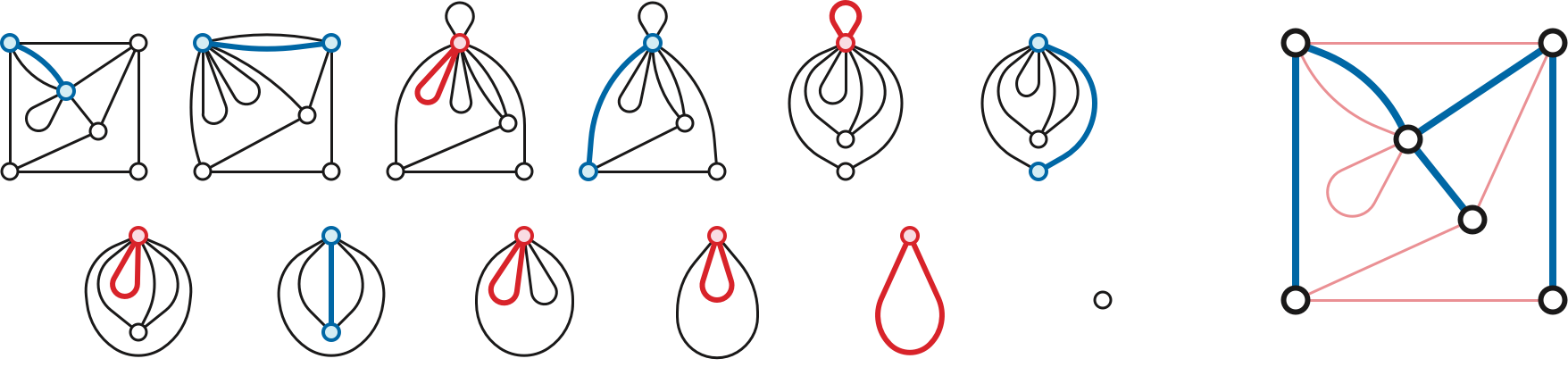
Equivalence of tree-cotree decompositions and tree-onion figures
Random (but not uniform!) rooted planar maps via random tree-onion figures
Well, okay, we only proved this formula for curves, but extending our inductive proof to multicurves requires us to consider only one additional case. Suppose some \(2\to0\) move disconnects a multicurve \(\Gamma\) into two smaller connected multicurves \(\Gamma^\sharp\) and \(\Gamma^\flat\). The original map \(\Gamma\) has \(n^\sharp + n^\flat + 2\) vertices and \(f^\sharp + f^\flat\) faces (including the deleted bigon and the common outer face), and the induction hypothesis implies that \(f^\sharp = n^\sharp + 2\) and \(f ^\flat = n^\flat+2\). Later we will see yet another proof of Euler’s formula (not on David’s list) based on Schnyder woods.↩︎
\(\dots\) on display in the bottom of a locked filing cabinet stuck in a disused lavatory with a sign on the door saying ‘Beware of the Leonhard’.↩︎
\(\dots\) and the formula isn’t Euler’s.↩︎