Let \(\Sigma = (V, E, F)\) be a planar map with outer face \(o\), where each edge \(e\) is assigned a non-negative weight \(w(e)\).1 Call any vertex incident to \(o\) a boundary vertex of \(\Sigma\). The multiple-source shortest-path problem asks for an implicit representation of the shortest paths from \(s\) to \(t\), for all boundary vertices \(s\) and all vertices \(t\). An explicit representation of these shortest paths, for example as a shortest-path tree rooted at every node on the outer face, requires \(\Omega(n^2)\) space in the worst case. Nevertheless, the multiple-source shortest-path problem can be solved in only \(O(n\log n)\) time, in any of the following forms:
Given a collection of \(k\) vertex pairs \((s_i, t_i)\), where each \(s_i\) is a boundary vertex, we can report all \(k\) shortest-path distances \(\textsf{dist}(s_i, t_i)\) in \(O(n \log n + k\log n)\) time.
Assuming the outer face \(o\) has \(k\) vertices, we can report the \(O(k^2)\) shortest-paths distances between every pair of boundary vertices in \(O(n\log n + k^2)\) time.
We can preprocess \(\Sigma\) in \(O(n\log n)\) time into a data structure using \(O(n\log n)\) space, that can report the shortest-path distance from an arbitrary boundary vertex to an arbitrary vertex in \(O(\log n)\) time.
The multiple-source shortest-path problem was first posed and solved by Philip Klein in 2005. Here I’m describing a slight simplification of Klein’s algorithm published by Sergio Cabello and Erin Chambers in 2007. This algorithm plays an essential role in several efficient algorithms for planar graphs and surface graphs.
The MSSP algorithm relies on a characterization of shortest paths developed by Lester For in the mid-1950s. Fix a source vertex \(s\). For each vertex \(v\), let \(\textsf{dist}(v)\) denote the shortest-path distance from \(s\) to \(v\). Let \(\textsf{pred}(v)\) denote the predecessor of vertex \(v\) (if any) in some shortest path from \(s\) to \(v\). Let \(T_s\) denote the tree of shortest paths from \(s\) to other vertices, defined so that \(\textsf{pred}(v)\) is the parent of \(v\) in \(T_s\). Finally, define the slack of each dart \(u\mathord\to v\) as \[ \textsf{slack}(u\mathord\to v) := \textsf{dist}(u) + w(u\mathord\to v) - \textsf{dist}(v) \] A dart whose slack is negative is called tense.
Ford’s generic single-source shortest path algorithm starts by assigning \(\textsf{dist}(s) = 0\) and tentatively assigning \(\textsf{dist}(v) = \infty\) for every vertex \(v\ne s\). Then as long as the graph contains at least one tense dart, the algorithm relaxes one tense dart \(u\mathord\to v\) by reassigning \(\textsf{dist}(v) \gets \textsf{dist}(u) + w(u\mathord\to v)\) and \(\textsf{pred}(v) \gets u\). When no more darts are tense, every value \(\textsf{dist}(v)\) is the correct shortest-path distance, and the predecessor pointers define a correct shortest-path tree \(T_s\).
To simplify presentation, I will assume for the rest of this presentation that for every vertex \(s\) and every vertex \(t\), there is a unique shortest path from \(s\) to \(t\). In particular, for each source vertex \(s\), there is a unique shortest-path tree \(T_s\) rooted at \(s\). At the end of this note I’ll describe two easy methods to enforce this assumption.
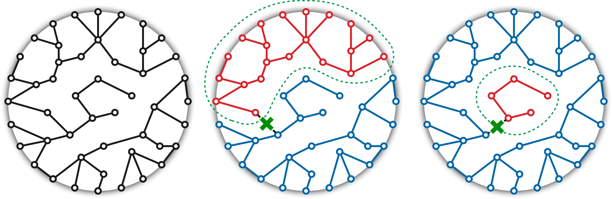
The dual subgraph \(C^* / e^*\) contains a cycle \(\gamma\) of length \(2\) that separates all vertices in \(U\) from all vertices in \(W\). If \(\gamma\) does not intersect \(B\), then \(U\) either contains every boundary vertex or none. Otherwise, \(\gamma\) intersects \(B\) exactly twice, so \(U\) contains an interval of boundary vertices. \(\qquad\square\)
Now suppose our original planar map \(\Sigma\) has \(k\) boundary vertices, indexed \(s_0, s_1, s_2, \dots, s_{k-1}\) in cyclic order. For each index \(i\), let \(T_i\) denote the shortest-path tree rooted at \(s_i\).
It follows that we can encode all \(k\) shortest paths using only \(O(n)\) space, either by recording the first and last trees \(T_i\) that contain each directed edge, or by recording the initial tree \(T_1\) followed by the differences \(T_2\setminus T_1, T_3\setminus T_2\dots T_k\setminus T_{k-1}\).
To solve the multiple-source shortest path problem, imagine moving the source vertex \(s\) continuously around the outer face and maintaining the shortest-path tree \(T_s\) rooted at \(s\). Although the shortest-path distances vary continuously as \(s\) moves, the structure of the shortest-path tree changes only at discrete events. (This approach is a variant of the parametric shortest-path problem first proposed by Karp and Orlin (1981).)
Now consider a single edge \(uv\) on the outer face. Suppose we have already computed the shortest-path tree \(T_u\) rooted at \(u\), and we want to maintain the shortest path tree \(T_s\) as the source vertex \(s\) moves along \(uv\) from \(u\) to \(v\). We insert \(s\) as a new vertex, partitioning \(uv\) into two edges \(us\) and \(sv\) with parametric weights \[ w_\lambda(us) = \lambda \cdot w(uv) \qquad\text{and}\qquad w_\lambda(sv) = (1-\lambda) w(uv) \] Every other edge \(xy\) has constant parametric weight \(w_\lambda(xy) = xy\). We then maintain the shortest-path tree \(T_\lambda\) rooted at \(s\), with respect to the weight function \(w_\lambda\), as the parameter \(\lambda\) increases continuously from \(0\) to \(1\). The initial shortest-path tree \(T_0\) is equal to \(T_u\), and the final tree \(T_1\) is equal to \(T_v\).
Fix a parameter value \(\lambda \in [0,1]\). For any vertex \(x\), let \(\textsf{dist}_\lambda(x)\) denote the shortest-path distance from \(s\) to \(x\) with respect to the weight function \(w_\lambda\). Similarly, for any dart \(x\mathord\to y\), let \[ \textsf{slack}_\lambda(x\mathord\to y) = \textsf{dist}_\lambda(x) + w_\lambda(x\mathord\to y) - \textsf{dist}_\lambda(y). \] Color each vertex \(x\) red if \(\textsf{dist}_\lambda(x)\) is an increasing function of \(\lambda\) (with derivative \(1\)), and blue if \(\textsf{dist}_\lambda(x)\) is an decreasing function of \(\lambda\) (with derivative \(-1\)). For generic values of \(\lambda\), every vertex except \(s\) is either red or blue. Finally, call a dart \(x\mathord\to y\) active if \(\textsf{slack}_\lambda(x\mathord\to y)\) is a decreasing function of \(\lambda\).
Without loss of generality, assume \(o = \textsf{left}(u\mathord\to v)\) is the outer face of \(\Sigma\). Let \(p = \textsf{right}(u\mathord\to v)\) be the other face incident to \(uv\). Let \(C^*_\lambda = (E\setminus T_\lambda)^*\) denote the spanning tree of \(\Sigma^*\) complementary to \(T_\lambda\). Finally, let \(\pi_\lambda\) denote the unique directed path in \(C^*_\lambda\) from \(o^*\) to \(p^*\).
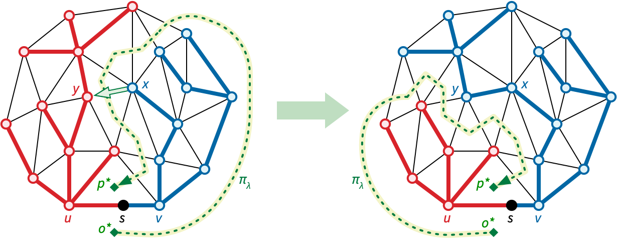
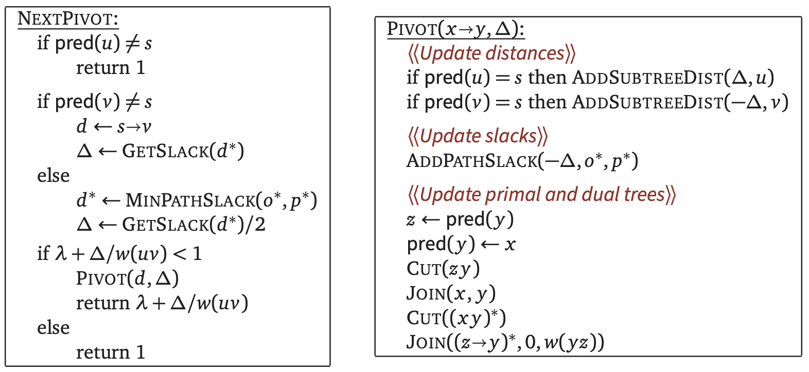
Thus, we can execute a single phase of the MSSP algorithm as follows. Initially, we set \(s = u\). We repeatedly find the tensest active dart \(d = x\mathord\to y\), move \(s\) distance \(\textsf{slack}(d)/2\) along \(uv\), increase all red distances and decrease all blue distances by \(\textsf{slack}(d)/2\), decrease the slacks of all active darts and increase the slacks of their reversals by \(\textsf{slack}(d)\), and finally pivot \(d\) into the tree by assigning \(\textsf{pred}(y) \gets x\). The loop ends either when there are no more active darts, or when the source vertex \(s\) reaches \(v\).
Each pivot changes at least one node \(y\) from red to blue, and no pivot changes any node from blue to red. Thus, once a dart is pivoted into the shortest-path tree, it is not pivoted out during that phase. Thus, the darts that are pivoted into the tree are precisely the darts in \(T_v \setminus T_u\). The disk-tree lemma now immediately implies that the total number of pivots over all phases is only linear.
To achieve a running time of \(O(n\log n)\), we need to perform each pivot quickly. We maintain both the shortest-path tree \(T_\lambda\) and the complementary dual spanning tree \(C^*_\lambda\) in data dynamic forest data structures that implicitly maintain dart values (slacks) or vertex values (distances) under edge insertions, edge deletions, and updates to the values in certain substructures.
We maintain the shortest path tree \(T_\lambda\) as a directed tree rooted at \(s\), with \(\textsf{dist}\) values associated with each vertex, in a data structure that supports the following operations:
\(\textsf{Cut}(x\mathord\to y)\): Remove the edge \(x\mathord\to y\) from \(T_\lambda\), breaking it into two rooted trees. The component containing \(x\) is still rooted at \(s\); the other component is rooted at \(y\).
\(\textsf{Link}(x, y)\): Add a directed edge from \(x\) to \(y\). This operation assumes that \(y\) a root. We always call \(\textsf{Link}\) immediately after \(\textsf{Cut}\) so that \(T_\lambda\) remains a single spanning tree.
\(\textsf{GetDist}(x)\): Return the distance value associated with vertex \(x\).
\(\textsf{AddSubtreeDist}(x)\): For every descendant \(y\) of \(x\), add \(\Delta\) to \(\textsf{dist}(y)\).
Similarly, we maintain the complementary dual spanning tree \(C^*_\lambda\) as an undirected unrooted tree, with \(\textsf{slack}\) values associated with every dart, in a data structure that supports the following operations.
\(\textsf{Cut}(xy)\): Remove the edge \(xy\) from \(C^*_\lambda\), breaking it into two trees.
\(\textsf{Link}(x, y, \alpha, \beta)\): Add the edge \(xy\) and assign \(\textsf{slack}(x\mathord\to y) = \alpha\) and \(\textsf{slack}(y\mathord\to x) = \beta\). We always call \(\textsf{Link}\) immediately after \(\textsf{Cut}\) so that \(C^*_\lambda\) remains a single dual spanning tree.
\(\textsf{GetSlack}(x\mathord\to y)\): Return the slack value associated with dart \(x\mathord\to y\).
\(\textsf{MinPathSlack}(\Delta, x, y)\): Return the \(d\) on the directed path from \(x\) to \(y\) such that \(\textsf{slack}(d)\) is minimized.
\(\textsf{AddPathSlack}(\Delta, x, y)\): For each dart \(d\) on the directed path from \(x\) to \(y\), add \(\Delta\) to \(\textsf{slack}(d)\) and subtract \(\Delta\) from \(\textsf{slack}(\textsf{rev}(d))\).
The self-adjusting top trees, proposed by Bob Tarjan and Renato Werneck in 2005, support all the operations we need for both data structures in in \(O(\log n)\) amortized time each. A description of self-adjusting top trees (or the splay trees they use under the hood) is unfortunately beyond the scope of this note (or this course).
With these data structures in hand, we can identify the tenses active dart and perform the necessary updates to pivot it into \(T_\lambda\) in \(O(\log n)\) amortised time. The following figure shows the algorithm to perform the next pivot, with all data structure operations in place. As we already argued, the total number of pivots is \(O(n)\), so the overall algorithm runs in \(O(n\log n)\) time, as claimed.
Cleaner to show only the generic case: both red and blue vertices.
Computing all \(k^2\) boundary-to-boundary distances \(O((n + k^2)\log n)\) time is straightforward.
The MSSP algorithm implicitly assumes that there is a unique shortest path between any two vertices of \(\Sigma\); in particular, for any source vertex \(s\), there is a unique shortest-path tree \(T_s\). More subtly, it also assumes that there is a unique tensest active dart. This assumption obviously does not hold in general, but we can enforce it if necessary using any of several standard perturbation techniques. I’ll describe two such techniques here, but there are other possibilities.
Standard perturbation methods either explicitly or implicitly define a secondary weight \(w’(u\mathord\to v)\) for each each dart \(u\mathord\to v\) in \(\Sigma\). The perturbed weight of a dart \(d\) is then defined as \[ \tilde{w}(d) := w(d) + w’(d)\cdot \varepsilon \] for some sufficiently small real number \(\varepsilon>0\). Rather than computing a particular value of \(\varepsilon\), we consider the limiting behavior as \(\varepsilon\) approaches zero. Thus, we can consider each perturbed weight \(\tilde{w}(d)\) to be an ordered pair or vector \[ \tilde{w}(d) := ( w(d), w’(d) ). \] We compute lengths of paths by summing these vectors normally, but we compare path lengths lexicographically. That is, we consider one path \(\pi\) to be shorter than another path \(\pi’\) if either of the following conditions holds:
The simplest perturbation method chooses random secondary weights for each edge. For example, if we choose each secondary weight \(w’(e)\) uniformly at random from the real interval \([0,1]\), then the lengths of all simple paths (indeed, the lengths of all finite walks) are distinct with probability \(1\).
Somewhat more realistically, the following lemma implies that we can choose small random integers for the secondary weights.
Isolation Lemma (Mulmuley, Vazirani, and Vazirani 1987): Let \(\mathcal{F}\) be any family of subsets of \([n]\). For each index \(i\in [n]\), let \(w’(i)\) be chosen independently and uniformly at random from \([N]\). Define the weight \(w’(S)\) of any subset \(S\subseteq[n]\) as \(w’(S) = \sum_{i\in S} w’(i)\). With probability at least \(1-n/N\), the minimum-weight set in \(\mathcal{F}\) is unique.
Corollary: If each perturbation weight \(w’(e)\) is chosen independently and uniformly at random from \([n^4]\), then with probability \(1 - 1/O(n)\), all shortest paths with respect to the perturbed weight function \((w, w’)\) are unique.
Let me emphasize that the Isolation Lemma only implies that shortest paths are distinct; other pairs of paths may still have equal length, even after perturbation.
Let \(T\sqcup C\) be a tree-cotree decomposition of \(\Sigma\). Root the dual spanning tree \(C^*\) at the dual of the outer face \(o^*\), and direct all edges of \(C^*\) away from the root. We define the weight \(w’(d)\) of each dart \(d\) of \(\Sigma\) as follows:
Equivalently, for any dart \(d\not\in T\), let \(\textsf{cycle}_T(d)\) be the unique directed cycle in \(T + d\). Then \(w’(d)\) is the number of faces of \(\Sigma\) inside \(\textsf{cycle}_T(d)\) if that cycle is oriented counterclockwise, the negation of the number of interior cycles if the cycle is clockwise, and zero if \(d\) is in \(T\).
The previous lemma implies that although the secondary weights \(w’\) depends on the choice of tree-cotree decomposition, the resulting shortest paths do not!
Figure!
First, suppose \(\pi\) and \(\pi’\) do not cross. Then the closed walk \(\pi - \pi’\) is a weakly simple closed curve, which implies that the non-zero winding numbers \(\textsf{wind}(\pi-\pi’, f)\) are either all \(1\) or all \(-1\). It follows that \(\textsf{wind}(\pi-\pi’, f) = 0\) for every face \(f\), which is only possible if \(\pi\) and \(\pi’\) use the same subset of edges. In other words, \(\pi = \pi’\).
Now suppose \(\pi\) and \(\pi’\) cross at some vertex \(x\). The prefixes \(\alpha = \pi[s, x]\) and \(\alpha’ = \pi’[s, x]\) must be shortest paths, otherwise we could shorten one of \(\pi\) and \(\pi’\). Similarly, the suffixes \(\beta = \pi[x,t]\) and \(\beta’ = \pi’[x,t]\) must be shortest paths. The inductive hypothesis now implies that \(\alpha = \alpha’\) and \(\beta = \beta’\). Again, we conclude that \(\pi = \pi’\). \(\qquad\square\)
In fact, we can implement cotree perturbation without explicit secondary weights. Suppose \(\pi\) and \(\pi’\) are two paths with the same endpoints. We say that \(\pi\) is to the left of \(\pi’\) if the closed walk \(\pi-\pi’\) winds negatively around at least one face, but does not wind positive around any face. If \(\pi\) is to the left of \(\pi\)’, we immediately have \(w’(\pi) < w’(\pi’)\).
It is not hard to show that for any two paths \(\pi\) and \(\pi’\) with the same endpoints, either one path is the left of the other, or a third path is to the left of both of them. Thus, shortest paths with respect to cotree perturbation are always leftmost shortest paths.
We can simulate cotree perturbation by always breaking ties to the left. In the MSSP algorithm, we always pivot the leafmost tensest active dart.
Need more details here
Cotree perturbation is attractive both because it is deterministic and because it can often be implemented implicitly, but its asymmetry can be a disadvantage. Unless shortest paths are already unique, cotree perturbation yields shortest paths that are not symmetric, even when the original graph is undirected. The reversal of the leftmost shortest path from \(s\) to \(t\) is the rightmost shortest path from \(t\) to \(u\). Thus, algorithms that rely on the usual behavior of undirected shortest paths cannot automatically use this technique.
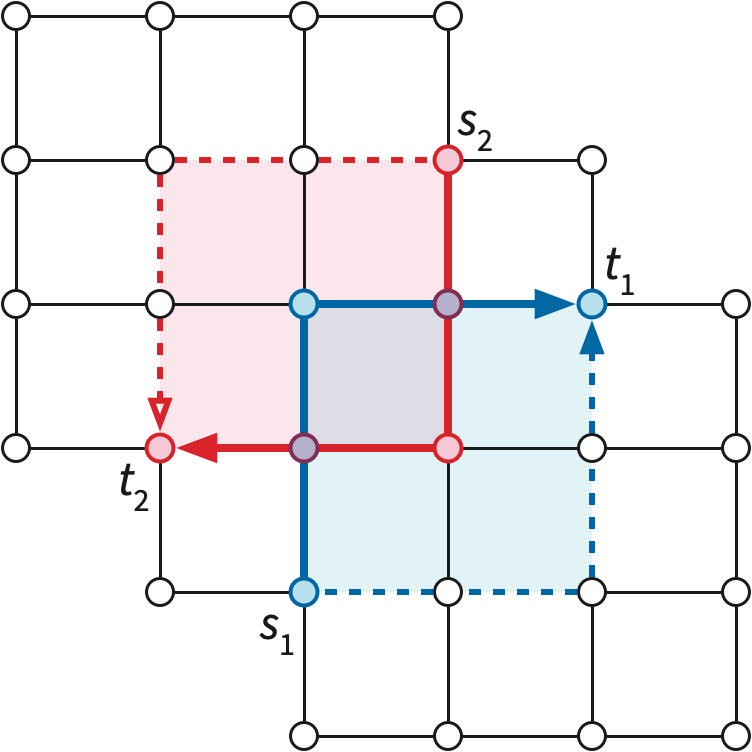
As a simple example, consider the non-crossing shortest paths problem. Given an undirected planar map \(\Sigma\) with weighted edges and several pairs of vertices \((s_1, t_1), \dots, (s_k, t_k)\) on the outer face, we want to compute shortest paths between each pair \(s_i\) and \(t_i\) that are pairwise non-crossing. If shortest paths in \(\Sigma\) are already unique, then it suffices to independently compute the shortest path in \(\Sigma\) from \(s_i\) to \(t_i\) for each index \(i\). But suppose the terminals appear in order \(s_1, t_1, s_2, t_2\) on the outer face, and we use cotree perturbation to enforce uniqueness. Then the shortest path from \(s_1\) to \(t_1\) might cross the shortest path from \(s_2\) to \(t_2\).
In fact the algorithm adapts easily to directed graphs, where a dart and its reversal may have different weights, but for ease of exposition, I’ll stick to undirected graphs in this note.↩︎