Let \(G\) be an arbitrary graph, and let \(s\) and \(t\) be two vertices of \(G\). An \((s, t)\)-cut (or more formally, an \((s,t)\)-edge-cut) is a subset \(X\) of the edges of \(G\) that intersects every path from \(s\) to \(t\) in \(G\). A minimum \((s,t)\)-cut is an \((s,t)\)-cut of minimum size, or of minimum total weight if the edges of \(G\) are weighted. (In this context, edge weights are normally called capacities.)
The fastest method to compute minimum \((s, t)\)-cuts in arbitrary graphs is to compute a maximum \((s, t)\)-flow and then exploit the classical proof of the maxflow-mincut theorem. In undirected planar graphs, however, this dependency is reversed; the fastest method to compute maximum flows actually computes minimum cuts first.
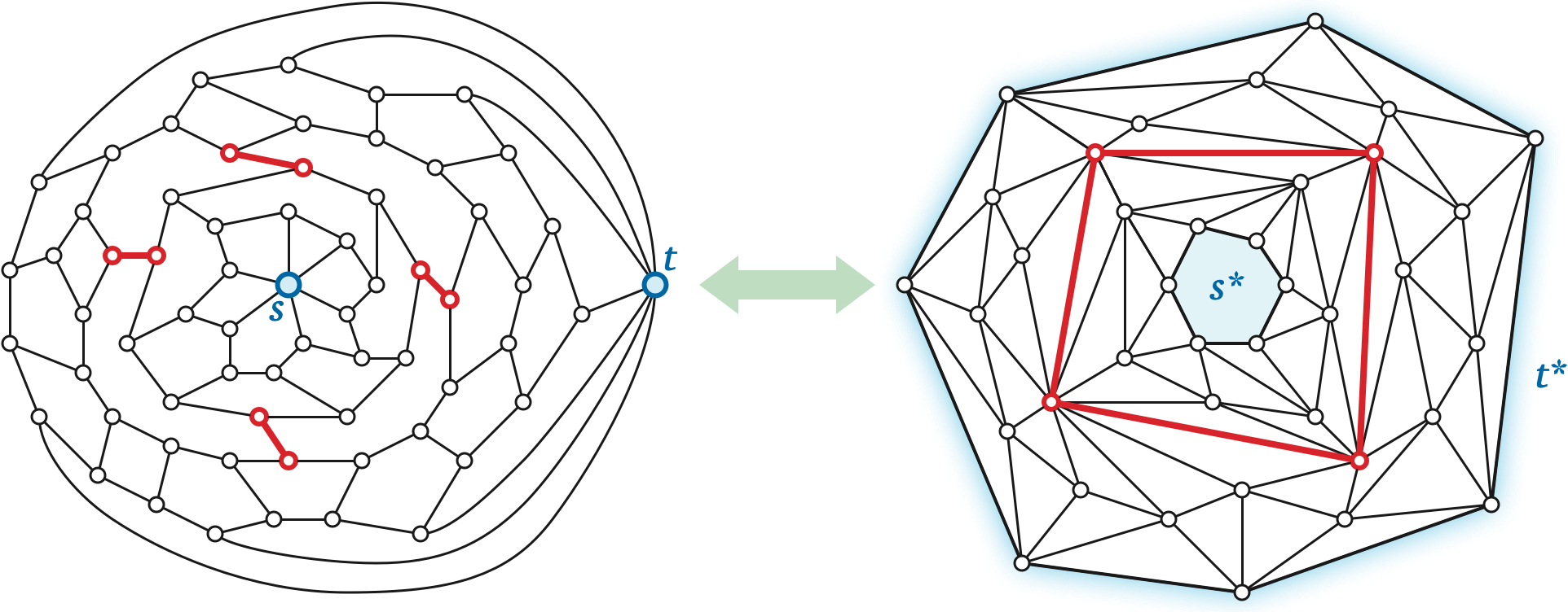
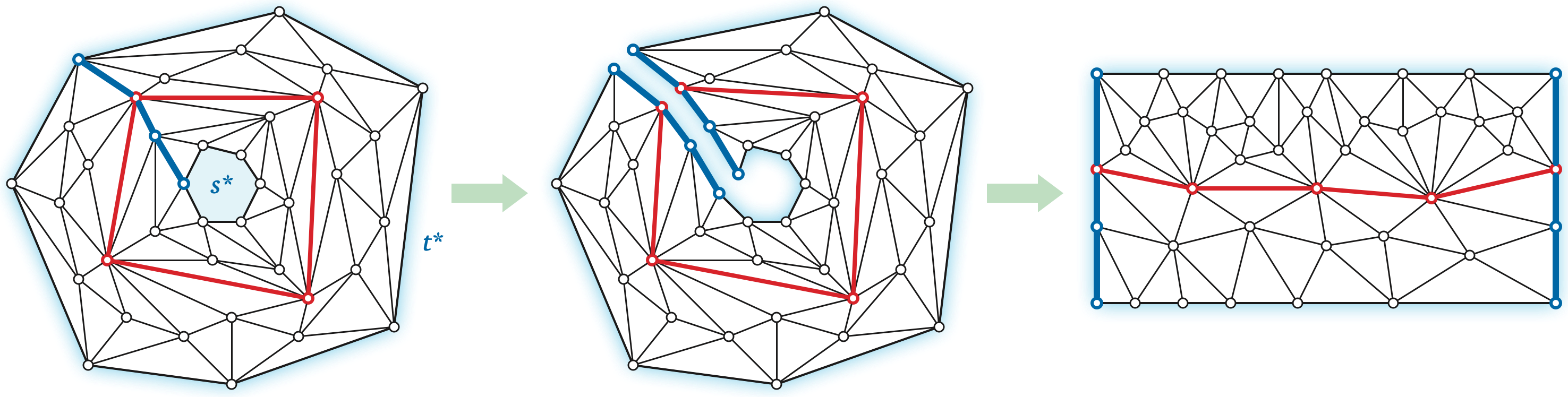
Let \(\Sigma\) be an undirected planar map, each of whose edges \(e\) has a non-negative capacity \(c(e)\), and let \(s\) and \(t\) be vertices of \(\Sigma\). The first step in our fast minimum-cut algorithm is to view the problem through the lens of duality. It is helpful to think of the source vertex \(s\) and the target vertex \(t\) as punctures or obstacles — points that are missing from the plane — and similarly to think of the corresponding faces \(s^*\) and \(t^*\) as holes in the dual map \(\Sigma^*\). In other words, we should think of the dual map \(\Sigma^*\) as a decomposition of the annulus \(A = \mathbb{R}^2 \setminus (s^*\cup t^*)\) rather than a map on the plane or a disk. Without loss of generality, assume that \(t^*\) is the outer face of \(\Sigma^*\).
A simple cycle \(\gamma\) in \(\Sigma^*\) is essential if it satisfies any of the following equivalent conditions:
Each edge \(e^*\) in the dual map \(\Sigma^*\) has a cost or length \(c^*(e^*)\) equal to the capacity of the corresponding primal edge \(e\). Whitney’s duality between simple cycles in \(\Sigma\) and and minimal cuts (bonds) in \(\Sigma^*\) immediately implies the following:
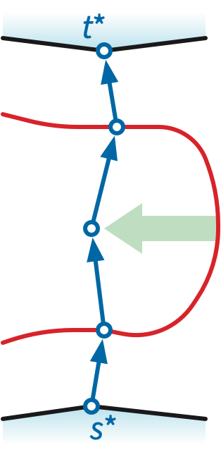
Now let \(\pi\) be a shortest path in \(\Sigma^*\) from any vertex of \(s^*\) to any vertex of \(t^*\). We can measure the winding number of any directed cycle \(\gamma\) in \(\Sigma^*\) by counting the number of times \(\gamma\) crosses \(\pi\) in either direction. We have to define “crossing” carefully here, because \(\gamma\) and \(\pi\) could share edges.
Suppose \(\pi = p_0\mathord\to p_1\mathord\to \cdots \mathord\to p_k\), where \(p_0\) lies on \(s^*\) and \(p_k\) lies on \(t^*\). To simplify the following definition, we add two “ghost” darts \(p_{-1}\mathord\to p_0\) and \(p_k\mathord\to p_{k+1}\), where \(p_{-1}\) lies inside \(s^*\) and \(p_{k+1}\) lies inside \(t^*\). We say that a dart \(q\mathord\to p_i\) enters \(\pi\) from the left (resp. from the right) if the darts \(p_{i-1}\mathord\to p_i\), \(q\mathord\to p_i\), and \(p_{i+1}\mathord\to p_i\) are ordered clockwise (resp. counterclockwise) around \(p_i\). Symmetrically, we say that a dart leaves \(\pi\) to the left (resp. to the right) if its reversal enters \(\pi\) from the left (resp. from the right). The same dart can leave \(\pi\) to the right and enter \(\pi\) to the left, or vice versa.
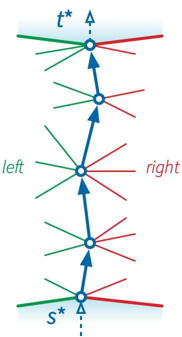
A positive crossing between \(\pi\) and \(\gamma\) is a subpath of \(\gamma\) that starts with a dart entering \(\pi\) from the right and ends with a dart leaving \(\pi\) to the left, and a negative crossing is defined similarly. Intuitively, for purposes of defining crossings, we are shifting the path \(\pi\) very slightly to the left, so that it intersects the edges of \(\Sigma^*\) transversely. It follows that the winding number \(\textsf{wind}(\gamma, s^*)\) is the number of darts in \(\gamma\) that leave \(\pi\) to the left, minus the number of darts in \(\gamma\) that enter \(\pi\) from the left.
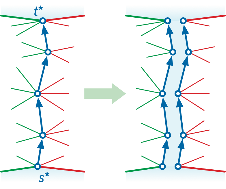
Now let \(\Delta := \Sigma^* \backslash\!\!\backslash \pi\) denote the planar map obtained by slicing the annular map \(\Sigma^*\) along path \(\pi\). The slicing operation replaces \(\pi\) with two copies \(\pi^+\) and \(\pi^-\). Then for every vertex \(p_i\) of \(\pi\), all edges incident to \(p_i\) on the left are redirected to \(p_i^+\), and all edges incident to \(p_i\) on the left are redirected to \(p_i^-\). The channel between two two paths \(\pi^+\) and \(\pi^-\) joins \(s^*\) and \(t^*\) into a single outer face. Thus, we should think of \(\Delta\) as being embedded on a disk. Every face of \(\Sigma^*\) except \(s^*\) and \(t^*\) appears as a face in \(\Delta\).
For any index \(i\), let \(\sigma_i\) denote the shortest path in \(\Delta\) from \(p_i^+\) to \(p_i^-\). The shortest essential cycle \(\gamma\) in \(\Sigma^*\) appears in \(\Delta\) as one of the shortest paths \(\sigma_i\). Thus, to compute the minimum \((s,t)\)-cut in our original planar map \(\Sigma\), it suffices to compute the length of every shortest path \(\sigma_i\) in \(\Delta\).
The simplest way to compute these \(k\) shortest-path distances is to run Dijkstra’s algorithm at each vertex \(p_i^+\). Assuming \(\pi\) has \(k\) edges, so there are \(k+1\) terminal pairs \(p_i^\pm\), this algorithm runs in \(O(kn\log n)\) time, which is \(O(n^2\log n)\) time in the worst case. We can reduce the running time to \(O(kn\log\log n)\) using the faster shortest-path algorithm we described in the previous lecture note, or even to \(O(kn)\) using a linear-time shortest-path algorithm.
Alternatively, we can compute all \(k\) of these shortest paths using a multiple-source shortest-paths algorithm. The parametric MSSP algorithms of Klein and Cabello et al. both require \(O(n\log n)\) time, which is faster in the worst case than \(O(kn)\), but slower when \(k\) is small. In particular, even when \(k=2\), that algorithm could require \(\Omega(n)\) pivots. The more recent recursive contraction algorithm runs in \(O(n\log n\log k)\) time if we use Dijkstra’s algorithm to compute shortest paths, or in \(O(n\log k)\) time if we use a linear-time shortest-path algorithm.
An older and simpler divide-and-conquer algorithm, proposed by John Reif in 1983, exactly matches the recursive contraction MSSP algorithm. Reif’s algorithm computes the median shortest path \(\sigma_m\), where \(m = \lfloor k/2 \rfloor\), and then recurses in each component of the sliced map \(\Delta \backslash\!\!\backslash \sigma_m\). One of these components contains the terminal pairs \(p_0^\pm, p_1^\pm, \dots, p^\pm_m\); the other contains the terminal pairs \(p_m^\pm, p_{m+1}^\pm, \dots, p_k^\pm\).
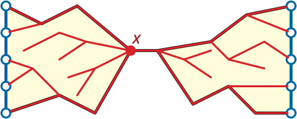
Reif’s algorithm falls back on Dijkstra’s algorithm in two base cases. First, if \(k\le 2\), we can obviously compute each of the \(k\) shortest paths directly. A more subtle base case happens when the “floor” and “ceiling” paths collide. Let \(\alpha\) denote the boundary path from \(p_0^+\) to \(p_0^-\), and let \(\beta\) denote the boundary path from \(p_k^+\) to \(p_k^-\). If \(\alpha\) and \(\beta\) share a vertex \(x\), then for every index \(i\) we have \(\textsl{dist}(p_i^+, p_i^-) = \textsl{dist}(p_i^+, x) + \textsl{dist}(x, p_i^-)\); thus, instead of recursing, we can compute all \(k\) shortest-path distances by computing a single shortest-path tree rooted at \(x\). (This second base case is not necessary for the correctness of Reif’s algorithm, but it is necessary for efficiency.)
Let \(T(n,k)\) denote the running time of Reif’s algorithm, where \(k+1\) is the number of terminal pairs and \(n\) is the total number of vertices in the map \(\Delta\). This function obeys the recurrence \[ T(n,k) = T(n_1, \lfloor k/2 \lfloor) + T(n_1, \lceil k/2 \rceil) + O(n\log n). \] where \(n_1\) and \(n_2\) are the number of vertices in the two components of \(\Delta \backslash\!\!\backslash \sigma_m\). The second base case ensures that each vertex and edge of \(\Delta\) appears in at most \(O(1)\) subproblems at any level of the recursion tree.1 Thus, the total work at any level of recursion is \(O(n\log n)\). The recursion tree has depth at most \(O(\log k)\), so the overall algorithm runs in \(O(n\log n\log k)\) time.
If we use a linear-time shortest-path algorithm instead of Dijkstra, the running time improves to \(O(n\log k)\). This improvement was first described by Greg Frederickson in 1987, as one of the earliest applications of \(r\)-divisions.
[[[This is still really sketchy!]]]
In the previous lecture note, we described a 2009 algorithm by Klein, Mozes, and Weimann to compute shortest paths in directed planar maps, possibly with negative dart lengths, in \(O(n\log^2 n)\) time. In 2010, Shay Mozes and Christian Wulff-Nilsen improved this algorithm even further by using a good \(r\)-division at each level of recursion (with \(r \approx n/\log n\)) instead of just one separator cycle; their improved algorithm runs in \(O(n\log^2n /\log\log n)\).
Recall the high-level description of the Klein-Mozes-Weimann algorithm:
Steps 1, 4, and 5 of Mozes and Wulff-Nilsen’s faster algorithm are identical. In step 2, the only minor different is that we need to run MSSP around the boundary of each hole of each piece, instead of just once around the sole cycle separator. The total time for each piece is \(O(r\log r)\), so the total time for this step across the entire \(r\)-division is \(O(n/r)\cdot O(r\log r) = O(n\log r)\).
The only major change to the algorithm is in step 3; we need to modify FR-Bellman-Ford to deal with holes in each piece of the \(r\)-division.
In step 2, we compute all boundary-to-boundary distances within each piece of the \(r\)-division using MSSP. Specifically, within each piece \(P\), we run MSSP around each of the \(O(1)\) boundary cycles of \(P\). The total time for each piece is \(O(r\log r)\), so the total time for this step across the entire \(r\)-division is \(O(n/r)\cdot O(r\log r) = O(n\log r)\).
Modifying step 3 is more interesting. Recall that a good \(r\)-division \(\mathcal{R}\) breaks \(\Sigma\) into \(O(n/r)\) pieces, each with \(O(r)\) vertices, \(O(\sqrt{r})\) boundary vertices, and \(O(1)\) holes; thus, overall, \(\mathcal{R}\) has \(O(n/\sqrt{r})\) boundary vertices, organized into \(O(n/r)\) cycles. We construct a complete directed multigraph \(\hat{R}\) over the boundary vertices of the \(r\)-division, with an edge \(u{\to}v\) with weight \(\textsf{dist}_P(u,v)\) for every piece \(P\) containing both \(u\) and \(v\).
Bellman-Ford computes shortest-path distances in \(\hat{R}\) in \(O(n/\sqrt{r})\) phases; in each phase, we find and relax all tense edges. Our modification of FR-Bellman-Ford breaks each relaxation phase into subphases:
for each piece P:
   for each boundary cycle S of P:
       for each boundary cycle T of P:
           relax every edge within P from S to T
We already described how to relax every edge in \(P\) from a boundary cycle to itself in \(O(k\alpha(k))\) time (or \(O(k)\) expected time). It remains to show how to relax all edges from one boundary cycle \(S\) to a different boundary cycle \(T\).
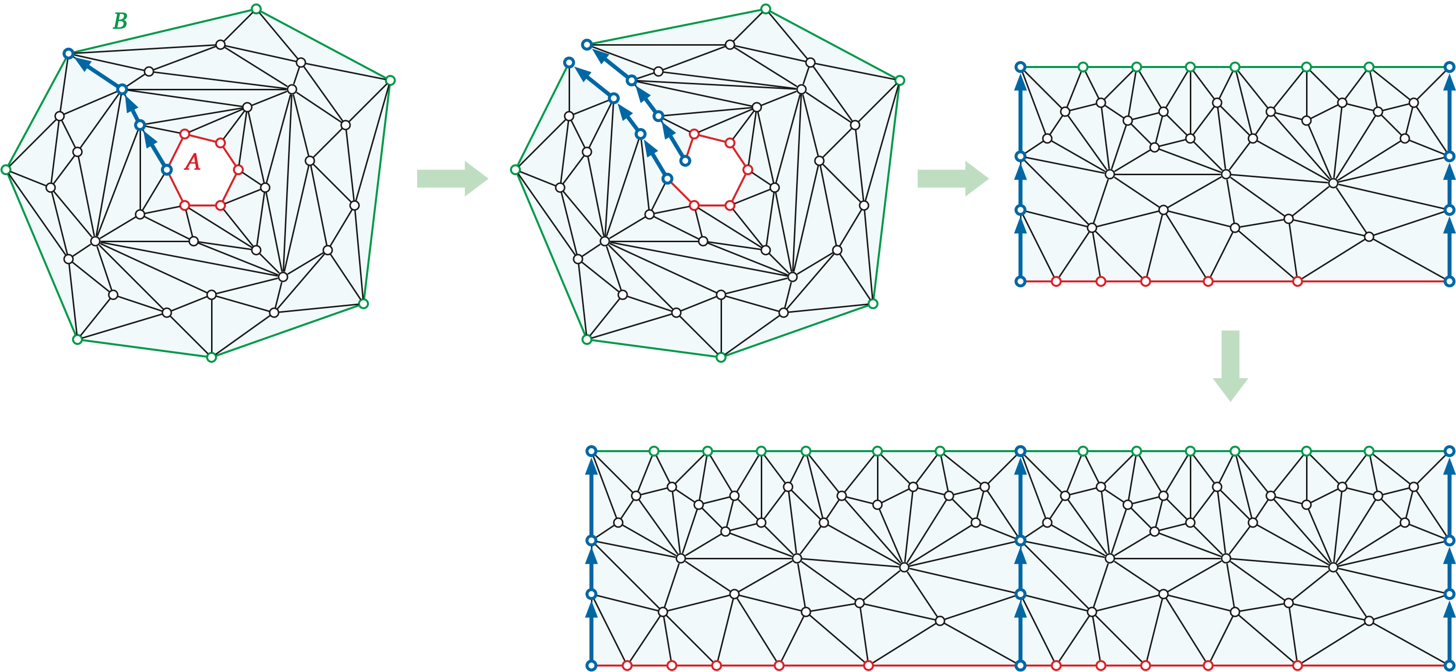
Without loss of generality, let’s assume that \(S\) and \(T\) are the only two boundary cycles in \(P\); we’ll treat any other boundary cycles as faces of \(P\). Thus, \(P\) is a map of an annulus. Let \(s_1, s_2, \dots, s_k\) and \(t_1, t_2, \dots, t_l\) denote the sequences of vertices of \(S\) and \(T\), respectively.
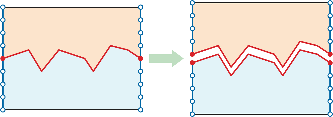
Let \(\pi\) be the shortest path in \(P\) from \(s_1\) to \(t_1\), and let \(\Delta = P \mathbin{\backslash\!\!\backslash} \pi\) be the map obtained by slicing \(\Sigma\) along the path \(\pi\). As before, the slicing operation duplicates the path \(\pi\) and merges the faces \(S\) and \(T\) into a single outer face.
Let \(\Delta’\) be a duplicate of \(\Delta\), and let \(\Delta^2\) denote the map obtained by gluing the “right” copy of \(\pi\) in \(\Delta\) to the “left” copy of \(\pi\) in \(\Delta’\).
Lemma: For all indices \(i\) and \(j\), we have \[\textsf{dist}_P(s_i,t_j) = \min\big\{ \textsf{dist}_{\Delta^2}(s_i,t_j),~ \textsf{dist}_{\Delta^2}(s’_i,t_j),~ \textsf{dist}_{\Delta^2}(a_i,b’_j) \big\}\].
[[[This is already claimed, but without proof, in the next lecture note.]]]
The matrix of distances from the “top edge” of \(\Delta^2\) to the “bottom edge” of \(\Delta^2\) is Monge! So we can relax all the edges from \(A\) to \(B\) in \(O(k+l)\) time with one invocation of SMAWK.
Suppose \(P\) has \(h = O(1)\) holes, with \(k_1, k_2, \dots, k_h\) boundary vertices; recall that \(k = \sum_i k_i = O(\sqrt{r})\). Then the total time to relax all boundary-to-boundary edges in \(P\) is \[ \sum_{i=1}^h O(k_i\alpha(k_i)) + \sum_{i=1}^h \sum_{j=1}^h O(k_i + k_j) ~=~ O(k\alpha(k) + kh) ~=~ O(\sqrt{r}\,\alpha(r)). \] It follows that the time to relax all edges of \(\mathcal{R}\) is \(O((n/\sqrt{r})\alpha(r)) = o(n)\)
Frederickson held the record for fastest planar minimum-cut algorithm for almost two and a half decades; the record was finally broken in 2011 by two independent pairs of researchers, who ultimately published their result jointly: Giuseppe Italiano, Yahav Nussbaum, Piotr Sankowski, and Christian Wulff-Nilsen. Their \(O(n\log\log n)\)-time algorithm relies on an improvement to Dijkstra’s algorithm in dense distance graphs, proposed by Jittat Fakcharoenphol and Satish Rao in 2001, and now usually called FR-Dijkstra.
Recall from the previous lecture on shortest paths that we can compute a dense distance graph for a nice \(r\)-division in \(O(n\log r)\) time. The dense distance graph has \(O(n/\sqrt{r})\) vertices—the boundary vertices of the pieces of the \(r\)-division—and \(O(n)\) edges. So Dijkstra’s algorithm with a Fibonacci heap runs in \(O(E + V\log V) = O(n + (n/\sqrt{r})\log n)\) time.
FR-Dijkstra removes the \(O(n)\) term from this running time. Specifically, within each piece of the \(r\)-division, the algorithm exploits the Monge structure in the boundary-to-boundary distances to avoid looking at every pair of boundary vertices. This is the same high-level strategy that we previously used with FR-Bellman-Ford, but with one significant difference: We do not know the relevant Monge arrays in advance. Instead, portions of each Monge array are revealed each time the Dijkstra wavefront touches the corresponding piece of the \(r\)-division.
I’ll discuss FR-Dijkstra in detail, along with the faster planar minimum-cut algorithm, in the next lecture.
Greg N. Frederickson. Fast algorithms for shortest paths in planar graphs with applications. SIAM J. Comput. 16(8):1004–1004, 1987.
Alon Itai and Yossi Shiloach. Maximum flow in planar networks. SIAM J. Comput. 8:135–150, 1979.
Giuseppe F. Italiano, Yahav Nussbaum, Piotr Sankowski, and Christian Wulff-Nilsen. Improved algorithms for min cut and max flow in undirected planar graphs. Proc. 43rd Ann. ACM Symp. Theory Comput., 313–322, 2011.
Shay Mozes and Christian Wulff-Nilsen. Shortest paths in planar graphs with real lengths in \(O(n \log^2 n/\log\log n)\) time. Proc. 18th Ann. Europ. Symp. Algorithms, 206–217, 2010. Lecture Notes Comput. Sci. 6347, Springer-Verlag. arXiv:0911.4963.
John Reif. Minimum \(s\)-\(t\) cut of a planar undirected network in \(O(n\log^2 n)\) time. SIAM J. Comput. 12(1):71–81, 1983.
Hassler Whitney. Non-separable and planar graphs. Trans. Amer. Math. Soc. 34:339–362, 1932.
Hassler Whitney. Planar graphs. Fund. Math. 21:73–84, 1933.
Without the second base case, it is possible for a constant fraction of the vertices to appear in a constant fraction of the recursive subproblems, leading to a running time of \(O(kn\log n)\).↩︎