Recall that a two-dimensional array \(M\) is Monge if the inequality \(M[i,j] + M[i’,j’] \le M[i’,j] + M[i,j’]\) holds for all indices \(i<i’\) and \(j<j’\). Any array where the columns are constant is Monge, and the sum of any two Monge arrays is Monge.
Suppose we are given a \(k\times k\) Monge array \(D\), and we are promised that there is a \(k\)-dimensional vector \(c\). Then no matter what values \(c\) contains, the array \(M\) defined by \(M[i,j] = D[i,j] + c[j]\) is Monge.
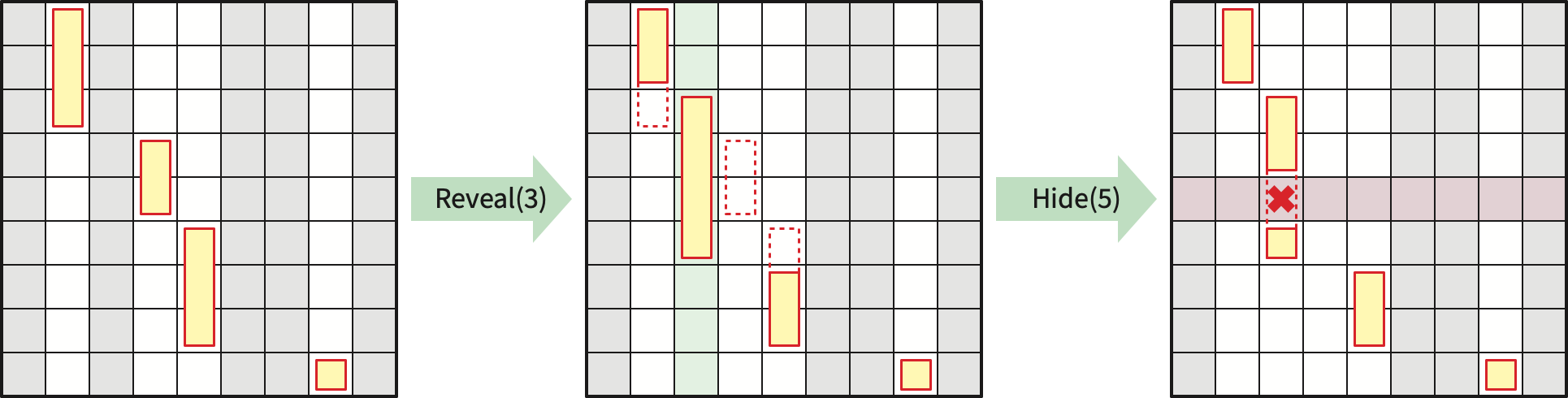
A Monge heap is a data structure that allows us to extract information from the array \(M\) as the coefficients of \(c\) are revealed. Specifically, a Monge heap supports the following three operations:
Over the lifetime of the data structure, we will \(\textsf{Reveal}\) at most \(k\) columns and \(\textsf{Hide}\) at most \(k\) rows.
An element of \(M\) is visible if its column has been \(\textsf{Reveal}\)ed but its row has not been \(\textsf{Hid}\)d\(\textsf{e}\)n. We call an element of \(M\) active if it is the smallest visible element in a visible row. Each visible column of \(M\) contains zero or more contiguous intervals of \(M\), which we call active intervals. Each active interval is specified by a triple of indices \((j, i_{\min}, i_{\max})\).
A Monge heap consists of three component data structures (described in more detail below):
These data structures support each \(\textsf{Reveal}\) in \(O(\log k)\) amortized time, \(\textsf{FindMin}\) in \(O(1)\) time, and \(\textsf{Hide}\) in \(O(\log k)\) time. Over the lifetime of the data structure, we call each of these operations at most \(k\) times, thereby finding the minimum elements in some subset of the rows of \(M\) in \(O(k\log k)\) time. (This is slower than the \(O(k)\) running time of SMAWK, but that algorithm requires the entire array \(M\) to be visible from the beginning.)
At all times, the submatrix (or minor) of visible elements in \(M\) is Monge. This implies that the minimum visible elements in the visible rows of \(M\) are monotone: The index of the row minimum is a non-decreasing function of the row index. More explicitly: For any indices \(i<i’\) of visible rows, if \(M[i,j]\) is the minimum (visible) element of row \(i\), and \(M[i’,j’]\) is the minimum (visible) element of row \(i’\), then \(j\le j’\).
Thus, each visible column \(j\) of \(M\) contains the smallest elements of a interval of visible rows, which may be broken into smaller intervals by hidden rows. Each live interval can be described by a triple of indices \((j, i_{\min}, i_{\max})\), indicating that \(M[i,j]\) is the minimum element in every row \(i\) such that \(i_{\min}\le i\le i_{\max}\), and moreover none of those rows has been hidden. The live intervals partition the visible rows of \(M\), so there are at most \(k\) of them at any time.
We maintain the live intervals \((j, i_{\min}, i_{\max})\) in a priority queue, implemented as a standard binary min-heap, where the priority of any interval is its smallest element. In particular, the smallest visible element in \(M\) is the priority of the live interval at the root of the heap, so we can support \(\textsf{FindMin}\) in \(O(1)\) time.
The smallest element in any live interval \((j, i_{\min}, i_{\max})\) depends only on the known Monge matrix \(D\). To compute these minimum elements quickly, we preprocess each column \(D[\cdot, j]\) into a data structure that supports range-minimum queries of the following form:
The range-minimum data structure consists of a static balanced binary search tree with \(k\) leaves. The \(i\)th leaf stores \(D[i,j]\), and every internal node stores the minimum value of its two children, along with the index of the leaf storing that value. This data structure is constructed once at the start of the algorithm, in \(O(k)\) time, and it answers any range-minimum query in \(O(\log k)\) time.
Whenever we \(\textsf{Insert}\) a new live interval \((j, i_{\min}, i_{\max})\) into the priority queue, we perform a range-minimum query to determine the priority of that interval. Thus, the overall \(\textsf{Insert}\)ion time is \(O(\log k)\). The other priority queue operations \(\textsf{ExtractMin}\) and \(\textsf{Delete}\) also take \(O(\log k)\) time.
\(\textsf{Reveal}(j, x)\) is implemented in \(O(\log k)\) amortized time as follows:
Find the live intervals \(I^- = (j^-, i_{\min}^-, i_{\min}^-)\) and \(I^+ = (j^+, i_{\min}^+, i_{\min}^+)\) immediately before and after \((j, \cdot, \cdot)\) in lexicographic order, in \(O(\log k)\) time, by querying the balanced binary search tree.
While \(M[i_{\min}^-, j] < M[i_{\min}^-, j^-]\), replace \(I^-\) with its predecessor in lexicographic order. Then binary search for the smallest index \(i_{\min}\) such that \(M[i_{\min}, j] < M[i_{\min}, j^-]\).
While \(M[i_{\min}^+, j] < M[i_{\min}^+, j^+]\), replace \(I^+\) with its successor in lexicographic order. Then binary search for the smallest index \(i_{\max}\) such that \(M[i_{\max}, j] < M[i_{\min}, j^+]\).
Delete any live intervals \((j^\pm, \cdot, \cdot)\) that overlap \((j, i_{\min}, i_{\max})\) from the priority queue.
Insert the new live intervals \((j, i_{\min}, i_{\max})\), \((j^-, \cdot, i_{\min}-1)\), and \((j^+, i_{\max}+1, \cdot)\) into the priority queue.
To obtain the claimed \(O(\log k)\) amortized time bound, we charge the time to delete any interval from the priority queue to its earlier insertion. The requirement that we only \(\textsf{Hide}\) rows when their minimum elements are visible implies that there is exactly one live interval in the \(\textsf{Reveal}\)ed column.
Finally, \(\textsf{Hide}(i)\) is implemented in \(O(\log k)\) time as follows:
Extract the live interval \((j, i_{\min}, i_{\max})\) from the root of the priority queue. Because row \(i\) contains the smallest visible element in \(M\), that smallest element is \(M[i,j]\) and \(i_{\min}\le i\le i_{\max}\).
Find the smallest element \(M[i,j]\) in that interval using a range-minimum query.
Insert the live intervals \((j, i_{\min}, i-1)\) and \((j, i+1, i_{\max})\) into the priority queue.
Suppose we are given a planar map \(\Sigma\) (called \(\Delta\) in the previous lecture) with non-negatively weighted edges. Recall that a nice \(r\)-division partitions \(S\) into \(O(n/r)\) pieces, each with \(O(r)\) vertices and \(O(\sqrt{r})\) boundary vertices, and each with the topology of a disk with \(O(1)\) holes.
Let \(D\) denote the array of boundary-to-boundary distances for a single piece \(R\) of this \(r\)-division. I claim that we can represent \(D\) using a small number of Monge arrays. We need to consider two types of boundary-to-boundary distances, depending on whether the two vertices lie on the same hole of \(R\) or on different holes.
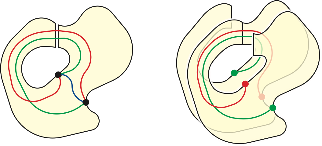
First, consider two holes in \(R\), with boundaries \(\alpha\) and \(\beta\). Think of \(R\) as a map on the annulus, with boundary cycles \(\alpha\) and \(\beta\). Let \(\pi\) be the shortest path from any vertex \(a_1 \in \alpha\) to any vertex \(b_1\in \beta\). For any vertices \(a_i\in \alpha\) and \(b_j\in \beta\), the shortest path in \(R\) from \(s\) to \(t\) either does not cross \(\pi\) at all, crosses \(\pi\) positively once, or crosses \(\pi\) negatively once. Let \(\Delta = R\setminus\!\!\setminus \pi\), and let \(\Delta^2\) be the map obtained by gluing two copies of \(\Delta\) together along \(\pi\), as shown in the figure below. Then we have \[ \textsf{dist}_R(a_i, b_j) = \min\left\{ \begin{gathered} \textsf{dist}_\Delta(a_i, b_j) \\[0.25ex] \textsf{dist}_{\Delta^2}(a_i^+, b_j^-) \\ \textsf{dist}_{\Delta^2}(a_i^-, b_j^+) \end{gathered} \right\} \] where \(v^+\) and \(v^-\) denote the two copies of vertex \(v\) in \(\Delta^2\). Thus, the array \(D(\alpha,\beta)\) of pairwise distances between vertices of \(\alpha\) and vertices of \(\beta\) is the element-wise minimum of three Monge arrays.
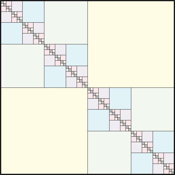
Next consider a single hole in \(R\) with boundary \(\alpha\); by construction \(\alpha\) has at most \(O(\sqrt{r})\) vertices. As we saw two lectures ago, the array \(D(\alpha)\) of pairwise distances in \(R\) between vertices in \(\alpha\) is almost Monge. Instead of splitting this array into partial Monge arrays, we recursively partition it into \(O(\sqrt{r})\) square Monge subarrays. Specifically, the upper right and lower left quadrants of \(D(\alpha)\) are both Monge, and we recursively subdivide the lower left and upper right quadrants. Every row or column of \(D(\alpha)\) intersects at most \(O(\log r)\) of these square subarrays. The total perimeter of these Monge arrays is \(O(\sqrt{r} \log r)\).
Putting these two cases together, we can represent the boundary-to-boundary distances within each piece \(R\) using \(O(\sqrt{r})\) Monge arrays, with total area \(O(r)\) and total perimeter \(O(\sqrt{r}\log r)\). Altogether there are \(O(n/\sqrt{r})\) Monge arrays associated with the entire \(r\)-division, with total area \(O(n)\) and total perimeter \(O((n/\sqrt{r})\log r)\).
Finally, suppose we associate a Monge heap with every Monge array in every piece of our \(r\)-division. Then the total number of \(\textsf{Reveal}\) and \(\textsf{Hide}\) operations we can perform is \(O((n/\sqrt{r})\log r)\), and each of those operations takes \(O(\log r)\) amortized time. Thus, the total time spent constructing and maintaining all Monge heaps, over their entire lifetimes, over the entire \(r\)-division, is \(O((n/\sqrt{r}) \log^2 r)\).
Fakcharoenphol and Rao implement their improvement to Dijkstra’s algorithm as follows. We begin by computing a nice \(r\)-division for \(\Sigma\) and the dense-distance graph for that \(r\)-division in \(O(n\log r)\) time, for some value of \(r\) to be determined later.
The query phase of FR-Dijkstra solves the single-source shortest path problem in the dense distance graph: Given a boundary vertex \(s\) in our \(r\)-division, compute the shortest-path distance to every other boundary vertex in the \(r\)-division. The algorithm mirrors the Dijkstra’s algorithm, but using a nested collection of heaps instead of a standard priority queue:
\(O(\sqrt{r})\) Monge heaps for each piece of the \(r\)-division, once for each Monge array in the decomposition described above.
A standard priority queue, called a piece heap, for each piece of the \(r\)-division, containing the minimum elements of every Monge heap associated with that piece. We automatically update the piece heap whenever the minimum element of a Monge heap changes.
A standard priority queue, called the global heap, containing the minimum elements of the piece heaps. We automatically update the global heap whenever the minimum element of a piece heap changes.
To begin the algorithm, we initialize all the component heaps to empty, call \(\textsf{Reveal}(s, 0)\) and \(\textsf{Hide}(s)\) inside every Monge heap containing the source vertex \(s\). In alter iterations, whenever we extract the next closest vertex \(v\) from the global priority queue, we call \(\textsf{Reveal}(v, \textsf{dist}(v))\) and \(\textsf{Hide}(v)\) in every Monge heap containing vertex \(v\). By induction, the vertex at the top of the global heap is always the closest boundary vertex beyond the current Dijkstra wavefront.
The running time of the algorithm is dominated by the time spent maintain the three different levels of heaps.
As we argued above, the total time spent managing all Monge heaps is \(O((n/\sqrt{r}) \log^2 r)\).
For each piece \(R\), we perform \(O(\log r)\) operations in \(R\)’s piece heap for each boundary vertex of \(R\). Thus, the number of piece-heap operations across the entire \(r\)-division is \(O((n/\sqrt{r}) \log r)\); each piece-heap operation takes \(O(\log r)\) time.
Finally, each iteration of Dijkstra’s algorithm removes one vertex \(v\) from the global heap and performs at most one deletion and one inserti on for each piece containing \(v\). Said differently, for each piece \(R\), we perform \(O(1)\) global-heap operations for boundary vertex of \(R\). So the total number of global-heap operations is \(O(n/\sqrt{r})\); each global-heap operation takes \(O(\log n)\) time.
Thus, the overall running time of the query phase of FR-Dijkstra is \(O((n/\sqrt{r})(\log^2r + \log n))\). (The final \(\log n\) term can be eliminated with more effort.)
In the previous lecture, we reduced computing minimum \((s,t)\)-cuts to the following problem. Given a planar map \(\Sigma\) with non-negatively weighted weighted edges, and vertices \(s_0, s_1, \dots, s_k, t_k, \dots, t_1, t_0\) in cyclic order on the outer face, compute the shortest path distance \(\textsf{dist}(s_i, t_i)\) for every index \(i\). Reif’s algorithm solves this problem in \(O(n\log k)\) time by computing the median shortest path \(\pi_m\) from \(s_m\) to \(t_m\), where \(m=\lfloor k/2 \rfloor\), and then recursing on both sides of the sliced map \(\Sigma \backslash\!\!\backslash \pi_m\).
The more efficient algorithm of Italiano et al. follows Reif’s divide-and-conquer strategy, in three phases.
In the initialization phase, we construct a nice \(r\)-division of \(\Sigma\), construct its dense distance graph by running MSSP in each piece, and initialize the range-minimum trees needed to support FR-Dijkstra. This phase runs in \(O(n\log r)\) time.
Let \(\lambda = \lfloor \log_2 k \rfloor\). In the coarse divide-and-conquer phase, we compute shortest paths from \(s_{i\lambda}\) to \(t_{i\lambda}\) for all indices \(0\le i\le \lfloor i/\lambda \rfloor\), using Reif’s divide-and-conquer strategy, using FR-Dijkstra to compute each shortest path.
Finally, in the fine divide-and-conquer phase, we run Reif’s algorithm within each of the \(O(k/\lambda)\) slabs left by the previous phase, using the linear-time shortest path algorithm to compute each shortest path. Since each slab has only \(\lambda = O(\log k)\) terminal pairs on its boundary, the total time for this phase is \(O(n\log\log k)\).
Crudely, the coarse divide-and-conquer phase stops after \(O(\log(k/\lambda)) = O(\log n)\) levels of recursion, and the total time spent at each level is \(O((n/\sqrt{r})(\log^2r + \log n))\) time at each level. It follows that the overall time for this phase is \(O((n/\sqrt{r})(\log^2r + \log n)\log k) = O((n/\sqrt{r})\log^3 n)\), and thus the overall running time of the overall algorithm is \[ O\left(n\log r + \frac{n}{\sqrt{r}}\log^3 n + n\log \log k\right). \] Setting \(r = \log^6 n\) gives us a final running time of \(O(n\log\log n)\). (With more effort, this time bound can be reduced to \(O(n\log\log k)\).)
The previous high-level description and analysis overlooks several technical details which are crucial for the efficiency of the algorithm. Here I’ll give only a brief sketch of the most significant outstanding issues and how to resolve them.
Arguably the most significant detail is that the pieces of the \(r\)-division do not respect the slab boundaries. The the running time of the query phase of FR-Dijkstra within any slab depends on the total size of all pieces that intersect that slab, and a single piece could intersect several (or even all) slabs at any level of recursion. To avoid blowing up the running time, we must slice pieces (and their underlying collections of Monge arrays) along the shortest paths we compute. This can be done.
Just as in Reif’s algorithm, we stop the course recursion early whenever any vertex of the dense-distance graph appears on both the “floor” and “ceiling” paths of a slab. All \(s_i\)-to-\(t_i\) distances through that slab will be computed in \(O(n)\) time in the fine phase of the algorithm. If we ignore these collapsed slabs, then at every level of recursion, each boundary vertex appears in at most two slabs, so the sum over all sub-pieces of the number of boundary nodes in that sub-piece is in fact \(O(n/\sqrt{r})\).
Another important technical detail is that after the coarse phase ends, we need to translate the shortest paths in the dense-distance graph into explicit shortest paths in \(\Sigma\). In particular, we need to translate each boundary-to-boundary distance within a single piece, as computed by MSSP, into an explicit boundary-to-boundary path. If we record the execution of the MSSP algorithm as a persistent data structure, we can extract the last edge of the shortest path from any boundary node \(s\) to any internal node \(v\) in \(O(\log\log\deg(v))\) time. Thus, a shortest path consisting of \(\ell\) edges can be extracted in \(O(\ell\log\log n)\) time. If we assume (as Italiano et al. do) that
These \(O(k/\log k)\) shortest paths in \(\Sigma\) can overlap; in the worst case, the sum of their complexities is \(\Omega(nk/\log k)\). The union of these \(O(k/\log k)\) shortest paths is a forest \(F\); Italiano et al. describe how to compute \(F\) in \(O(n\log\log n)\) time.
Finally, at the beginning of the fine phase of the algorithm, suppose the floor \(\alpha\) and ceiling \(\beta\) of some slab coincide. We can compute the endpoints \(x\) and \(y\) of the shared path \(\alpha\cap\beta\) by performing least-common-ancestor queries in the forest \(F\). Then every \(s_i\)-to-\(t_i\) shortest path in that slab consists of the shortest path from \(s_i\) to \(x\), the unique path in \(F\) from \(x\) to \(y\), and the shortest path from \(y\) to \(t_i\). Thus, we can compute all \(s_i\)-to-\(t_i\) distances in that slab in linear time, by computing shortest path trees at \(x\) and \(y\).