Homotopy in Surface Maps

There’s not a lot in this section about algorithms, but there is a lot of important structure. Everything described in this note is based on tree-cotree decompositions.

Recall from the previous lecture that a tree-cotree decomposition of a surface map \(\Sigma\) is a partition of the edges \(E\) into three disjoint subsets \(T\sqcup L\sqcup C\), where

• \(T\) is a spanning tree of \(\Sigma\),
• \(C^*\) is a spanning tree of the dual map \(\Sigma^*\), and
• \(L = E\setminus (C\cup T)\) is the set of leftover edges.

Every surface map has a tree-cotree decomposition \((T,L,C)\). In fact, we can choose either the spanning tree \(T\) or the complementary dual spanning tree \(C\) arbitrarily, just as we did for tree-cotree decompositions of planar maps.

More generally, suppose we modify a map \(\Sigma\) by repeatedly either (1) contracting an arbitrary non-loop edge or (2) deleting an arbitrary non-isthmus edge, until eery edge is both a loop and an isthmus. Let \(T\) be the set of contracted edges, let \(V\) be the set of deleted edges, and let \(L\) be the final set of isthmus-loops (loop-isthmuses?). Then \((T,L,C)\) is a tree-cotree decomposition of the original map \(\Sigma\).

Equivalently, suppose we color the edges of \(\Sigma\) red, green, or blue in arbitrary order so that (1) every cycle contains at least one blue edge, (2) every edge cut contains at least one red edge, and (3) an edge is green if and only if it cannot be colored either red or blue. Then the red, green, and blue edges respectively define the spanning tree, leftover edges, and spanning cotree of a tree-cotree decomposition.

[[[Figure! Running example on a genus-2 map?]]]

Cut Graphs

A cut graph of a map \(\Sigma\) on surface \(\mathcal{S}\) is any subgraph \(X\) of \(\Sigma\) such that \(\mathcal{S} \setminus X\) an open topological disk. (Let me emphasize that here \(\setminus\) means to remove the points from the space, not merely deleting the edges from the map.)

Alternatively, we can define cut graphs in terms of a generalization of the slicing operation we already saw in the context of separators and minimum cuts. Slicing a map \(\Sigma\) along a subgraph \(X\) produces a new map \(\Sigma\mathbin{\backslash\!\!\backslash} X\) which contains \(\deg_X(v)\) copies of every vertex \(v\) of \(X\), two copies of every edge of \(X\), and at least one new face in addition to the faces of \(\Sigma\). By convention, we think of the faces of \(\Sigma\mathbin{\backslash\!\!\backslash} X\) that are not faces of \(\Sigma\) as holes that are missing from the surface; thus, \(\Sigma\mathbin{\backslash\!\!\backslash} X\) is always a map of a surface with boundary. At least intuitively, \(\Sigma\mathbin{\backslash\!\!\backslash} X\) is the map obtained by gluing together the faces of \(\Sigma\) along every edge that is not in \(X\). Then a cut graph of \(\Sigma\) is any subgraph \(X\) such that \(\Sigma\mathbin{\backslash\!\!\backslash} X\) is a closed disk.

[[[Figure]]]

For any tree-cotree decomposition \((T,L,C)\) of \(\Sigma\), the subgraph \(T\cup L\) is a cut graph of \(\Sigma\). Typically the cut graph \(X = T\cup L\) will contain several vertices with degree \(1\); removing any such vertex from \(X\) yields a smaller cut graph. A reduced cut graph is a cut graph with no degree-1 vertices at all; equivalently, a reduced cut graph is a minimal subgraph \(X\) such that \(\Sigma \mathbin{\backslash\!\!\backslash} X\) is a disk. We can reduce any cut graph by repeatedly removing degree-1 vertices until none are left.¹

In any surface map with Euler genus \(\bar{g} = 2-\chi > 1\), every reduced cut graph can be further decomposed into at most \(2\bar{g}-2\) cut paths between at most \(3\bar{g}-3\) vertices with degree at least \(3\), called branch points. In particular, if every branch point has degree exactly \(3\), there are exactly \(3\bar{g}-3\) branch points and \(2\bar{g}-2\) cut paths. (The only two exceptional surfaces are the projective plane (non-orientable genus \(1\)), where every reduced cut graph is a single one-sided cycle, and the sphere (orientable genus \(0\)), where by convention every reduced cut graph is a single vertex.)

[[[Figure!]]]

Systems of Loops and Homotopy

Fix an arbitrary vertex \(x\), called the basepoint. For each vertex \(v\), let \(\textsf{path}(v)\) denote the unique directed path in the spanning tree \(T\) from \(x\) to \(v\). For every dart \(d\), let \(\textsf{loop}(d)\) denote the following directed closed walk: \[ \textsf{loop}(d) := \textsf{path}(\textsf{tail}(d)) \cdot d \cdot \textsf{rev}(\textsf{path}(\textsf{head}(d))). \] Notice that \(\textsf{loop}(\textsf{rev}(d)) = \textsf{rev}(\textsf{loop}(d))\).

Finally, let \(\mathcal{L} = \{ \textsf{loop}(e^+) \mid e\in L \}\), where \(e^+\) denotes an arbitrary reference dart for edge \(e\). The set \(\mathcal{L}\) is called a system of loops for \(\Sigma\).

Recall that two closed curves in some space \(X\) are (freely) homotopic if one curve can be continuously deformed into the other on \(X\). Similarly, two paths in \(X\) with the same endpoints are homotopic if one path can be continuously deformed into the other while keeping the endpoints fixed. A system of loops gives us the necessary structure to decide whether two curves are homotopic, similarly to the “fences” in our planar homotopy-testing algorithm.

What’s a “curve”?

But before we can start talking concretely about algorithms, we have to nail down the phrase “given two curves” and “given a surface”. Our planar homotopy algorithm assumes that input curves are given as polygons, specified as a sequence of vertex coordinates; while it is possible to impose coordinates on surfaces that would permit a natural generalization of “polygons”, imposing geometry is almost always both wasteful and unnecessary.²

It is usually simpler and more efficient to treat curves on surfaces purely combinatorially, representing surfaces as maps (using rotation systems or reflection systems), and representing curves using one of two natural combinatorial models:

• Traversal: We consider only curves that are walks in the graph of \(\Sigma\); curves cannot intersect faces, and if a curve intersects an edge, it must traverse that edge monotonically from one end to the other. We can represent any such curve as an alternating sequence of vertices and darts (directed edges). If the edges of \(\Sigma\) are weighted, the length of a curve \(\alpha\) is the sum of the weights of the edges that \(\alpha\) traverses, counted with appropriate multiplicity.

• Crossing: We consider only curves that intersect the edges of \(\Sigma\) transversely, away from the vertices, and whose intersection with each face of \(\Sigma\) is simple (injective). We can represent any such curve as an alternating sequence of faces and knives (oriented edges). If the edges of \(\Sigma\) are weighted, the length of a curve \(\alpha\) is the sum of the weights of the edges that \(\alpha\) crosses, counted with appropriate multiplicity.

These two models are clearly dual to each other; a crossing curve in \(\Sigma\) is equivalent to—or more formally, IS—a traversing curve in the dual map \(\Sigma^*\), and vice versa. Which curve model we choose is strictly a matter of convenience. For the rest of this lecture, I’ll use the traversal model.

Spur and Face Moves

Even though we do not allow the input curves to intersect the interiors of faces, we cannot impose the same restriction on homotopies. Recall that we can think of any homotopy as a continuously deforming curve. Even though the deforming curve starts and ends on the vertices and edges of \(\Sigma\), it may pass through faces in some or all intermediate stages.

However, just as with generic curves in the plane, it turns out that any homotopy between traversal curves in surface maps can be decomposed into a finite sequence of combinatorial moves, of two types:

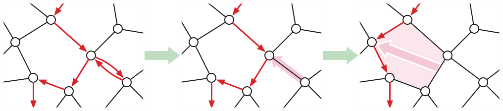
• A spur move either inserts or deletes a subpath consisting of a dart followed by its reversal; we call such a subpath a spur (or sometimes a spike).

• A face move replaces a subpath of the boundary of some face \(f\) with the complementary subpath on the boundary of \(f\).

Thus, asking whether a closed walk \(W\) in some map \(\Sigma\) is contractible is a purely combinatorial problem: Is there a sequence of spur and face moves that transforms \(W\) into a trivial walk?

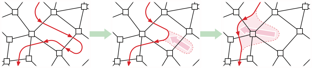
There is a dual pair of homotopy moves for crossing curves. The dual of a spur move, called a bigon move, deforms the curve to either insert or remove two consecutive crossings of the same edge. The dual of a face move, called a vertex move, deforms the curve across one vertex.

Characterizing Homotopy

Lemma: Let \((T,L,C)\) be an arbitrary tree-cotree decomposition of a surface map \(\Sigma\), and let \(x\) be a vertex of \(\Sigma\). Every directed walk from \(x\) to \(x\) in \(\Sigma\) is homotopic to a directed walk from \(x\) to \(x\) in the cut graph \(T\cup L\).

Proof:

It suffices to prove that any dart \(d\) in \(C\) (or more formally, any dart whose edge is in \(C\)) is homotopic to a walk in \(T\cup L\) from \(\textsl{tail}(d)\) to \(\textsl{head}(d)\).

Consider the fundamental domain \(\Delta = \Sigma \mathbin{\backslash\!\!\backslash} (T\cup L)\). The dart \(d\) is a boundary-to-boundary chord through the interior of \(\Delta\). Using a sequence of face moves, we can deform \(d\) to a path \(\pi\) around the boundary of \(\Delta\) from \(\textsf{tail}_\Delta(d)\) to \(\textsf{head}_\Delta(d)\). This boundary path \(\pi\) projects to a walk in the cut graph \(T\cup L\) from \(\textsf{tail}_\Sigma(d)\) to \(\textsf{head}_\Sigma(d)\). \(\qquad\square\)

Let \(\mathcal{L}^*\) denote the set of all loops formed by concatenating a finite sequence of loops in \(\mathcal{L}\) and their reversals. That is, \(\ell \in \mathcal{L}^*\) if and only if one of the following recursive conditions is satisfied:

• \(\ell\) is the empty loop
• \(\ell = \textsf{loop}(e^+) \cdot \ell’\) for some edge \(e\in L\) and some loop \(\ell’ \in \mathcal{L}^*\).
• \(\ell = \textsf{loop}(e^-) \cdot \ell’\) for some edge \(e\in L\) and some loop \(\ell’ \in \mathcal{L}^*\).

Lemma: Let \((T,L,C)\) be an arbitrary tree-cotree decomposition of a surface map \(\Sigma\), and let \(x\) be a vertex of \(\Sigma\). Every directed walk from \(x\) to \(x\) in \(\Sigma\) is homotopic to a loop in \(\mathcal{L}^*\).

Proof:

In light of the previous lemma, it suffices to consider only walks in the cut graph \(T\cup L\). Consider the closed walk \(w = v_0{\to}v_1{\to}v_2{\to}\cdots{\to}v_L\), where \(v_0 = v_L = x\). We easily observe that \(w\) is homotopic to the concatenation of paths \[ \begin{aligned} \textsf{path}(v_0) \cdot v_0{\to}v_1 \cdot \textsf{rev}(\textsf{path}(v_1)) &\cdot \textsf{path}(v_1) \cdot v_1{\to}v_2 \cdot \textsf{rev}(\textsf{path}(v_2)) \cdots \\ &\cdots \textsf{path}(v_{i-1}) \cdot v_{i-1}{\to}v_i \cdot \textsf{rev}(\textsf{path}(v_i)) \cdots \\ &\cdots \textsf{path}(v_{L-1}) \cdot v_{L-1}{\to}v_L \cdot \textsf{rev}(\textsf{path}(v_L)) \\ = \textsf{loop}(v_0{\to}v_1) \cdot \textsf{loop}(v_1{\to}v_2) \cdots & \textsf{loop}(v_{i-1}{\to}v_i) \cdots \textsf{loop}(v_{L-1}{\to}v_L) \end{aligned} \] because the initial path \(\textsf{path}(v_0)\) and final path \(\textsf{rev}(\textsf{path}(v_L))\) are both empty, and every intermediate path through \(T\) is immediately followed by its reversal.

Thus, it suffices to argue that every fundamental loop \(\textsf{loop}(d)\) is homotopic to a loop in \(\mathcal{L}^*\). Again, in light of the previous lemma, there are only two cases to consider:

• If \(|d|\in L\), then by definition either \(\textsf{loop}(d) \in \mathcal{L}\) or \(\textsf{rev}(\textsf{loop}(d)) = \textsf{loop}(\textsf{rev}(d)) \in \mathcal{L}\).

• Suppose \(|d| \in T\). Then \(\textsf{loop}(d) = \textsf{path}(v) \cdot \textsf{rev}(\textsf{path}(v))\), where \(v\) is one of the endpoints of \(d\), so we can deform \(\textsf{loop}(d)\) to the empty loop, through a finite sequence of spur moves. \(\qquad\square\)

[[[Figure!]]]

This lemma does not uniquely characterize homotopy classes of loops; in fact, every loop based at \(x\) is homotopic to infinitely many loops in \(\mathcal{L}^*\). In the next lecture, we’ll develop an efficient algorithm to decide whether two loops are homotopic, in effect by defining a canonical loop in \(\mathcal{L}^*\) for each homotopy class.

References

Aptly Named Sir

• Pants decompositions (except possibly in passing)