About These Exercises
These exercises are meant entirely for your own practice, understanding, and potentially future research. I will not ask you to submit solutions. I strongly encouraged everyone to discuss these problems (and any related questions that you come up with) on the course discussion forum.
Problems that I’m sure are open are labeled (!!). Problems that I don’t know how to solve, but that I’m not confident are open, are labeled (?). Labeled problems may or may not be difficult or interesting. Some exercises stray outside recent class material, either into the future or outside the class entirely; feel free to ask for clarification on Ed Discussion.
Some “open” problems on topics we haven’t covered yet may have been solved since the last time I taught this class. I’ll update relevant problems as the semester progresses.
Somewhat counterintuitively, the Jordan curve theorem does not extend to open curves of the form \(\pi\colon \mathbb{R}\to\mathbb{R}^2\), even when those curves are piecewise-linear. Let’s define an infinite polygonal chain to be an open curve that passes through an infinite sequence of points \(\dots, p_{-2}, p_{-2}, p_0, p_1, p_2, \dots\), where for each index \(i\), the subpath from \(p_{i-1}\) to \(p_i\) is the straight line segment \(p_{i-1}p_i\). As usual, an open curve is simple if (as a function) it is injective.
Describe a simple infinite polygonal chain \(P\) such that \(\mathbb{R}^2\setminus P\) is connected. Give explicit coordinates for each vertex \(p_i\) as a function of its index \(i\).
Describe a simple infinite polygonal chain \(P\) such that \(\mathbb{R}^2\setminus P\) has two components. (This should be easy.)
Describe a simple infinite polygonal chain \(P\) such that \(\mathbb{R}^2\setminus P\) has three components.
Describe a simple infinite polygonal chain \(P\) such that \(\mathbb{R}^2\setminus P\) has four components.
(?) Prove that the complement \(\mathbb{R}^2\setminus P\) of any simple infinite polygonal chain has at most four components.
Call an infinite polygonal chain sane if every vertex \(p_i\) has coordinates between \(-U\) and \(U\), and every edge \(p_ip_{i+1}\) has length between \(1\) and \(U\), for some real number \(U\gg 1\). (The precise value of \(U\) isn’t important; what is important is that \(U\) is finite.) Describe sane simple infinite polygonal chains \(P_1\), \(P_2\), and \(P_3\) such that for each index \(i\), the complement \(\mathbb{R}^2\setminus P_i\) has \(i\) components.
(?) Prove that the complement \(\mathbb{R}^2\setminus P\) of any sane simple infinite polygonal chain has at most three components.
In class we saw a proof, originally due to Dehn and Lennes, that the interior of any simple polygon in the plane can be frugally triangulated by adding interior diagonals. The proof relies on the Jordan curve theorem. In this problem we consider several extensions of the polygon triangulation theorem to spaces where the Jordan curve theorem does not hold.
Let \(P\) be a simple polygon that lies entirely in the interior of the unit square \(\square = [0,1]^2\). Prove that the area between \(\square\) and \(P\) can be triangulated. Every vertex of the triangulation must be a vertex of either \(P\) or \(\square\).
More generally, let \(P_0, P_1, P_2, \dots, P_k\) be pairwise-disjoint simple polygons such that the interior of \(P_0\) contains all the other polygons, but otherwise the interiors are disjoint. Prove that the area between \(P_0\) and the other polygons \(P_i\) (usually called a polygon with holes) can be triangulated using only line segments between the vertices of the various polygons.
A spherical polygon is a circular sequence of points connected by great-circle arcs on the sphere. A spherical polygon is simple if it does not self-intersect. The Jordan curve theorem implies that any spherical polygon \(P\) divides the sphere into two components, both of which are bounded. Prove that it is possible to triangulate both of these components using great-circle arcs between vertices of \(P\).
The infinite cylinder is the product \(S^1 \times\mathbb{R}\) of the circle and a line. Prove that any geodesic polygon on the infinite cylinder can be triangulated.
Prove that any geodesic polygon on the projective plane \(S^2 / \sim\) can be triangulated.
Prove that any geodesic polygon on the flat square torus \(S^1\times S^1\) can be triangulated.
For any simple polygons \(P\) and \(Q\), the Dehn-Schönflies theorem implies that there is a homeomorphism \(\phi \colon \mathbb{R}^2 \to \mathbb{R}^2\) such that \(\phi(P) = Q\). Moreover, if \(P\) has \(n\) vertices \(p_1,p_2,\dots,p_n\) and \(Q\) has \(n\) vertices \(q_1,q_2,\dots,q_n\), we can further require that \(\phi(p_i) = q_i\) for every index \(i\). This exercise asks you to construct such a homeomorphism explicitly.
Let \(\Box\) be a square that is large enough to comfortably contain both \(P\) and \(Q\). We say that a triangulation \(T\) of \(\Box\) supports \(P\) if every vertex of \(P\) is a vertex of \(T\) and every edge of \(P\) is the union of edges of \(T\). (Unlike the previous problem, vertices of \(T\) are not required to be vertices of \(P\) or \(\Box\).) Two triangulations \(T_P\) and \(T_Q\) of \(\Box\) with labeled vertices are compatible with \(P\) and \(Q\) if they satisfy the following conditions:
\(T_P\) and \(T_Q\) are isomorphic as labeled planar maps. That is, the vertex labeling induces bijections between the vertices, edges, and faces of \(T_P\) and the vertices, edges, and faces of \(T_Q\), respectively.
Corresponding vertices on the boundary of \(\Box\) have the same coordinates in both triangulations.
\(T_P\) supports \(P\), and \(T_Q\) supports \(Q\).
The vertex labeling also induces bijections between the vertices, edges, and interior faces of \(P\) and the vertices, edges, and interior faces of \(Q\), respectively. In particular, for any index \(i\), vertices \(p_i\) and \(q_i\) have the same label in \(T_P\) and \(T_Q\), respectively.
Describe an algorithm to compute compatible triangulations for two given \(n\)-gons with at most \(O(n^2)\) vertices. (This implies a piecewise-linear homeomorphism \(\phi\colon\mathbb{R}^2\to\mathbb{R}^2\) with complexity at most \(O(n^2)\) that is the identity outside the bounding box \(\Box\).)
Prove that the \(O(n^2)\) upper bound cannot be improved in the worst case.
(?) Describe an efficient algorithm to determine if two simple \(n\)-gons have compatible triangulations with exactly \(n+4\) vertices, namely, the vertices of the polygon plus the vertices of the bounding box \(\Box\). (I’m reasonably confident that this problem can be solved in polynomial time.)
(!!) Prove that computing compatible triangulations with the minimum number of vertices is NP-hard.
(!!) Describe an algorithm that either computes triangulations of the flat square torus that are compatible with two given geodesic polygons \(P\) and \(Q\), or correctly reports that no such triangulation exists. (A compatible triangulation exists if and only if \(P\) and \(Q\) are either both contractible or both essential.) How many vertices are required in the worst case?
It may be easier to start by considering compatible triangulations only of the interiors of the polygons, as described by Aronov, Seidel, and Souvaine [CGTA 1993]. A similar problem for arbitrary point sets was previously considered by Saalfeld [SOCG 1989]. Lubiw and Mondal [CCCG 2017, TCS 2020] recently proved that finding compatible triangulations for two polygons with holes with a minimum number of vertices is NP-hard.
The lecture notes offer two different definitions of the winding number of a polygon \(P\) around a point \(o\):
Prove that these two definitions are in fact equivalent. (Hint: Triangulate \(P\).)
Tired of the simple centuries-old game of Fast and Loose that everyone already knows, con artists Tenn and Peller are trying to develop more complex variants.
In their first variant, they plan to place the chain on the table so that it forms three loops, and then invite the mark to put fingers into two of them. The mark wins if the chain is held fast to the table by their two fingers. Placing fingers in all three loops must hold the chain fast to the table. Describe how Tenn and Peller can always win. Equivalently, describe a closed curve \(C\) in the plane and three points \(p,q,r\) such that \(C\) is contractible in \(\mathbb{R}^2\setminus\{p,q\}\) and in \(\mathbb{R}^2\setminus\{p,r\}\) and in \(\mathbb{R}^2\setminus\{q,r\}\), but not contractible in \(\mathbb{R}^2\setminus\{p,q,r\}\). How long is the crossing sequence of your curve?
In the harder variant, they place the chain so that it forms \(n\) loops, and then invite a crowd of marks to place fingers into any \(n-1\) of them. Equivalently, they want to want to design a curve that is non-contractible in the plane minus \(n\) points, but that becomes contractible if we ignore any one of those \(n\) points. The crossing sequence of your curve should be a small polynomial in \(n\).
See “Picture-Hanging Puzzles” by Demaine et al. [TCS 2013] for a different framing of this problem. For a more formal treatment, see Gartside and Greenwood [Fund. Math. 2007].
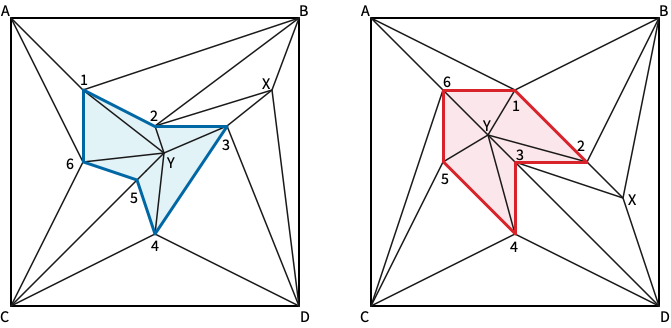
Fix an arbitrary point \(o\) in the plane, called the origin. Let \(P\) be a polygon in the punctured plane \(\mathbb{R}^2\setminus \{o\}\) with vertices \(p_0, p_1, \dots, p_{n-1}\). A vertex move on \(P\) replaces an arbitrary vertex \(p_i\) with a new point \(q_i\). This vertex move is safe if it preserves the widing number of the polygon around the original, that is, neither of the triangles \(\triangle p_i q_i p_{i-1}\) and \(\triangle p_i q_i p_{i+1}\) contains \(o\). (All index arithmetic is modulo \(n\).) A sequence of safe vertex moves describes a homotopy between two polygons with the same number of vertices and the same winding number around the origin.
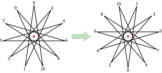
Let \(P\) and \(Q\) be two arbitrary polygons in \(\mathbb{R}^2\setminus \{o\}\) with the same number of vertices \(n\) and the same winding numer around the origin. Describe how to transform \(P\) into \(Q\) using \(O(n)\) safe vertex moves. [Hint: Aim for a canonical polygon with the correct winding number; the star polygon in part (a) may not be the best candidate.]
(!!) Now let \(O\) be a finite set of obstacle points in the plane, and let \(P\) and \(Q\) be homotopic polygons in \(\mathbb{R}^2\setminus O\) with the same number of vertices. How many safe triangle moves are necessary and sufficient to transform \(P\) into \(Q\) in the worst case? (Even the case \(k=2\) appears to be open.)
(!!) Finally, let \(P\) and \(Q\) be two arbitrary polygons in \(\mathbb{R}^2\) with the same number of vertices \(n\) and the same rotation number. Now call a vertex move dull if it preserves the rotation number of the polygon; that is, as vertex \(p_i\) moves, the angle \(\angle p_{i-1} p_i p_{i+1}\) is never zero. (Mnemonically, the corner is never sharp.) Is it always possible to transform \(P\) into \(Q\) using \(O(n)\) dull vertex moves?
(!!) Describe an efficient algorithm to generate a random curve (up to isotopy) with a given number of vertices, drawn uniformly from the set of isotopy classes. Existing algorithms either require exponential time or don’t even approximate the uniform distribution well.
(!!) In class we saw an algorithm of Steinitz to simplify an arbitrary generic planar curve with \(n\) vertices using \(O(n^2)\) homotopy moves. Moreover, Steinitz’s homotopy is monotone, meaning the number of vertices of the evolving curve never increases. Chang and Erickson described an algorithm that uses only \(O(n^{3/2})\) homotopy moves, but these can include \(0\to 2\) moves; they also proved a matching worst-case \(\Omega(n^{3/2})\) lower bound.
Can every curve be monotonically simplified using a sub-quadratic number of homotopy moves? Or is there a quadratic lower bound? (There is a quadratic lower bound if the homotopy is require to avoid even a single obstacle point.)
(!!) In class we saw a efficient algorithm, morally due to Gauss, Nagy, and Dehn, to determine whether a given unsigned Gauss code describes a curve in the plane; Tarjan and Rosenstiehl improved the running time of this algorithm to \(O(n)\).
Is there a polynomial-time algorithm to recognize unsigned Gauss codes of curves on more complex surfaces? Even the special case of the torus is open.
Exponential time is easy: Try all possible signings of the given Gauss code. Several characterizations are known, but all of them lead to exponential-time algorithms.
It may be easier to recognize Gauss codes of codes with special topological properties, such as null-homologous curves, contractible curves, curves in minimal position, or curves homotopic to a simple curve. As far as I know all these variants are open.
More ambitiously, how quickly can we determine the minimum-genus surface that supports a closed curve with a given unsigned Gauss code? Neither an efficient algorithm nor an NP-hardness result is known.
Let \(\Gamma = \{\gamma_1, \gamma_2, \dots, \gamma_k\}\) be a set of generic closed curves that intersect each other only pairwise, transversely, and away from their vertices; we call any such set a (generic) multicurve. For simplicity, assume that every curve \(\gamma_i\) is either non-simple or intersects another curve \(\gamma_j\). Then the image of \(\Gamma\) is a 4-regular plane graph, which may be disconnected. Conversely, every 4-regular plane graph is the image of a family of planar curves.
A Gauss paragraph of \(\Gamma\) is a sequence of \(k\) strings, obtained by uniquely labeling the vertices of \(\Gamma\), and then listing the vertices in order along each curve \(\gamma_i\) in an arbitrary direction, starting at an arbitrary basepoint, considering the curves in arbitrary order.
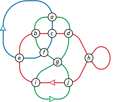
Now let’s go the other direction. A Gauss paragraph is any set of non-empty strings in which any symbol appears exactly twice or not at all. Each Gauss paragraph \(X\) defines a 4-regular undirected graph \(G(X)\) whose vertices are the characters in \(X\) and whose edges correspond to adjacent character pairs. If \(X\) is the Gauss paragraph of a family of planar curves, then \(G(X)\) is the image graph of that family.
Prove that if \(X\) is the Gauss paragraph of a family of planar curves, then the edges of \(G(X)\) can be directed so that every vertex has in-degree \(2\) and out-degree \(2\). (Consider self-intersection points of one curve and intersection points of two curves separately.)
Describe a linear-time algorithm that either directs the edges of \(G(X)\) as described in part (a) or correctly reports that no such orientation exists, given the Gauss paragraph \(X\) as input.
Prove that \(X\) is the Gauss paragraph of a generic family of planar curves if and only if \(G(X)\) has a planar embedding such that every component has a non-self-crossing Euler tour.
Sketch a linear-time algorithm to decide whether a given sequence of strings is the Gauss paragraph of a generic family of planar curves. (Just describe the necessary modifications to the algorithm for single curves.)
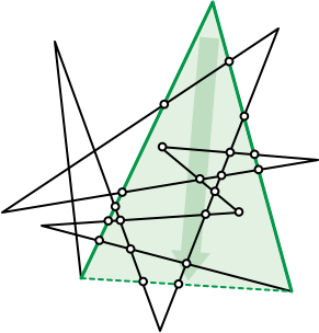
Let \(P\) be an arbitrary polygon with \(n\) vertices; for simplicity, assume no three vertices in \(P\) are collinear. The image graph \(G(P)\) is a planar straight-line graph whose nodes are the vertices of \(P\) and the intersection points of edges of \(P\). Let \(N\) denote the number of nodes in the image graph \(G(P)\). Trivially, \(n\le N\le \binom{n}{2}\).
We can easily reduce \(P\) to a triangle by repeated vertex deletion: replace some pair of edges \(p_{i-1} p_i p_{i+1}\) with a single edge \(p_{i-1}p_{i+1}\), deleting the shared vertex \(p_i\). Define the cost of deleting vertex \(p_i\) to be the number of nodes of \(G(P)\) that lie in the triangle \(\triangle p_{i-1}p_ip_{i+1}\), except for the three vertices \(p_{i-1}\), \(p_i\), and \(p_{i+1}\). For example, if \(P\) is convex, every vertex deletion has cost zero.
Prove that any vertex deletion with cost \(k\) can be transformed into a sequence of \(O(k)\) homotopy moves (\(1\leftrightarrow 0\), \(2\leftrightarrow 0\), or \(3\to 3\)), by treating the polygon as a generic curve. (Watch out for spurs!) This is the motivation for my definition of cost.
Trivially, every vertex deletion has cost \(O(n^2)\), and therefore any sequence of \(n-3\) vertex deletions has total cost \(O(n^3)\). Prove that this \(O(n^3)\) bound is tight in the worst case. (See problem 1.5!)
Prove that if \(P\) is simple, there is a sequence of \(n-3\) vertex deletions with total cost \(0\).
Prove that any polygon \(P\) can be reduced to a triangle by a sequence of \(n-3\) vertex deletions with cost \(O(N^2)\). (A vertex deletion can actually increase \(N\).)
(!!) Prove or disprove: There is a sequence of \(n-3\) vertex deletions with total cost \(O(N^{3/2})\). Your proof of part (b) implies a worst-case \(\Omega(N^{3/2})\) lower bound.
(!!) Let \(s, p_1, p_2, \dots, p_n\) be disjoint points in the plane. A proper squid is a collection of paths \(\pi_1, \pi_2, \dots, \pi_n\), where each path \(\pi_i\) connects \(s\) with the corresponding point \(p_i\), such that (1) the paths are simple and disjoint (except at \(s\)), and (2) the paths are incident to \(s\) in counterclockwise order \(\pi_1, \pi_2, \dots, \pi_n\).
A squid is a collection of paths from \(s\) to the points \(p_i\) that can be perturbed by an arbitrarily small distance into a proper squid.
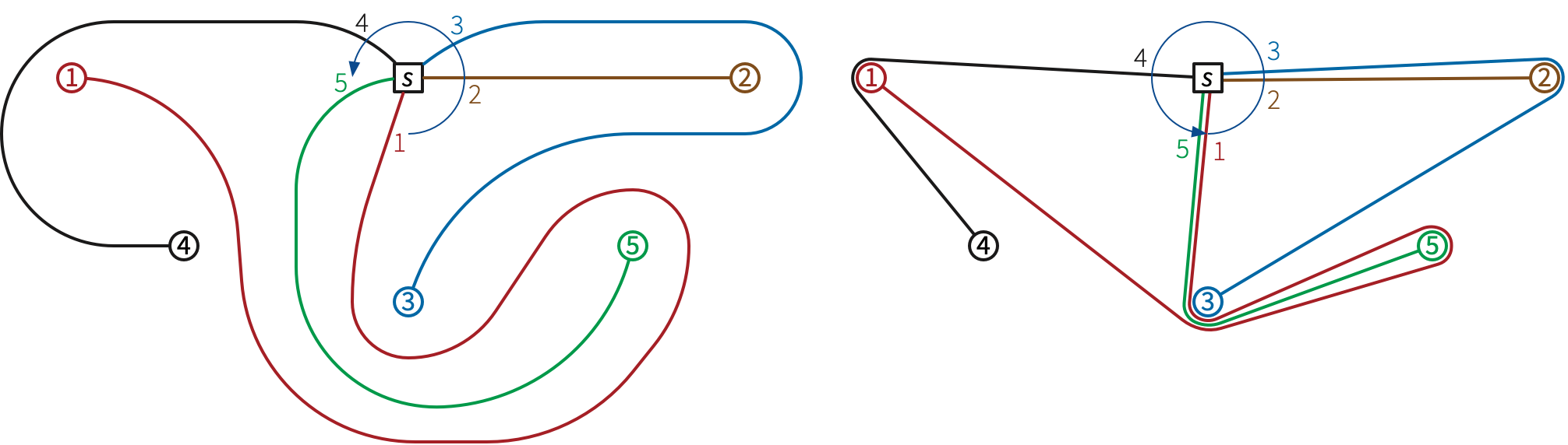
Either describe an algorithm for the following problem, or prove that it is NP-hard (or worse): Given points \(s, p_1, p_2, \dots, p_n\), find the minimum-length squid connecting those points. The minimum-length squid consists entirely of polygonal paths through the obstacle points \(p_j\).
I know how to solve this problem in exponential time. We can compute the minimum-length squid in a given homotopy class in polynomial time using the funnel algorithm; the hard part of the problem is finding the right homotopy class.
The problem is open even when all \(n+1\) points lie on a line.
Polyhedra are natural three-dimensional generalization of polygons, but they are surprisingly difficult to define precisely. In particular, formally defining regular polyhedra is remarkably subtle. It has been common knowledge for millennia that the five Platonic solids — tetrahedron, cube, octahedron, dodecahedron, and icosahedron — are the only regular polyhedra; we can find a proof in Euclid’s Elements (Book XIII, Proposition 18). But is that actually correct?
Here is one attempt at a reasonable definition. Let \(\Sigma = (V, E, F)\) be a finite planar map with vertices \(V\), edges \(E\), and faces \(F\). A polyhedral realization of \(\Sigma\) is a function assigning coordinates to vertices so that (1) the endpoints of each edge map to distinct points, and (2) the vertices of each face (including the outer face) map to coplanar points. Informally, \(\pi\) maps each edge of \(\Sigma\) to a line segment and each face of \(\Sigma\) to a polygon in some plane in \(\mathbb{R}^3\). A polyhedron is a polyhedral realization of a finite planar map. We call the images of \(V\), \(E\), and \(F\) the vertices, edges, and faces of the polyhedron.
Just like polygons, polyhedra are not required by definition to be simple. In particular, polyhedra can have overlapping features, including coincident vertices, collinear intersecting edges, and coplanar intersecting faces. However, for purposes of this exercise, I’m requiring polyhedra to be images of finite planar maps.
A flag in a planar map or a polyhedron is any triple \((v,e,f)\), where \(v\) is an endpoint of edge \(e\) and \(e\) is an edge of face \(f\). A planar map is regular if it has a flag-transitive automorphism group. That is, for any two flags \((v,e,f)\) and \((v',e',f')\), there is an bijection \(\alpha\colon\Sigma\to\Sigma\) such that \(\alpha(v) = v'\) and \(\alpha(e)=e'\) and \(\alpha(f) = f'\). Finally, a polyhedron is regular if, for any two flags, there is a rotation or reflection of \(\mathbb{R}^3\) that maps one flag to the other. In particular, the underlying planar map of any regular polyhedron is regular.
Give a complete list of all finite regular planar maps.
Give a complete list of all regular polyhedra. (Hint: There are more than five.)
(!!) Suppose we remove the word “planar” from the definition of polyhedron. Give a complete list of all regular polyhedra under this more general definition.
(!!!) Suppose we remove the word “finite” from the definition of polyhedron (but we keep “planar”). Give a complete list of all regular polyhedra under this more general definition.
(!!!!) Suppose we remove both “finite” and “planar” from the definition of polyhedron. Give a complete list of all regular polyhedra under this more general definition.
Prove the following facts about planar graphs and maps with \(n\) vertices.
So far we’ve seen two simple representations of closed curves in the plane: polygons (specified by vertex coordinates) and generic curves (specified by signed Gauss codes or rotation systems). Another natural representation is as closed walks in embedded graphs.
Let \(\Sigma\) be a fixed combinatorial planar map, called the scaffold, represented by a rotation system and a choice of outer face. Recall that a closed walk in \(\Sigma\) is a circular sequence of darts \(W = (d_0, d_1, \dots, d_\ell)\) such that \(\textsf{head}(d_i) = \textsf{tail}(d_{(i+1)\bmod \ell})\) for every index \(i\).
Describe a fast algorithm to compute an Alexander numbering for a given closed walk \(W\) in \(\Sigma\). For each face \(f\) of \(\Sigma\), your algorithm should compute the winding number of \(W\) around and point in \(f\). (Why are winding numbers independent of the geometry of \(\Sigma\)?)
A spur in a closed walk is an adjacent pair of darts \(d_i,d_{i+1}\) such that \(d_{i+1} = \textsf{rev}(d_i)\). Describe an algorithm to compute the rotation number of a spur-free closed walk in \(\Sigma\). (Why is the rotation number independent of the geometry of \(\Sigma\)?)
Suppose several bounded faces \(f_1, \dots, f_h\) of \(\Sigma\) are specified as holes. Describe an algorithm to decide whether two closed walks \(W\) and \(W’\) in \(\Sigma\) are homotopic in \(\mathbb{R}^2 \setminus (f_1\cup \cdots \cup f_h)\).
None of your algorithms should compute an actual geometric embedding of \(\Sigma\); instead, they should work directly with the rotation system.
When we think about algorithms for planar graphs, it is often useful to make assumptions about the degrees of vertices and/or the degrees of faces. Let \(\Sigma\) be a simple undirected planar map with weighted edges.
We can assume without loss of generality that every face of \(\Sigma\) has degree \(3\), by inserting diagonals into any higher-degree face. Moreover, we can preserve shortest-path distances by giving these new edges infinite weight (length), and we can preserve maximum flow values by giving the new edges weight (capacity) zero.
On the other hand, we can assume without loss of generality that every vertex of \(\Sigma\) has degree 3, by expanding each higher-degree vertex into a tree of degree-3 vertices (or equivalently, by triangulating faces in the dual graph \(\Sigma^*\)). Moreover, we can preserve shortest-path distances by giving these new edges weight (length) zero, and we can preserve maximum flow values by giving the new edges infinite weight (capacity).
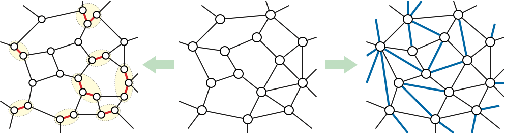
Unfortunately, triangulating faces increases vertex degrees, and expanding vertices increases face degrees; these two assumptions seem to cancel each other out. What if we need both vertices and faces to have small degree?
Prove that for some constants \(\Delta\), \(\Delta^*\), and \(c\), any simple \(n\)-vertex planar graph \(\Sigma\) can be modified by inserting and expanding edges into a new simple planar map \(\tilde\Sigma\) with at most \(cn\) vertices, such that each vertex of \(\tilde\Sigma\) has degree at most \(\Delta\) and each face of \(\tilde\Sigma\) has degree at most \(\Delta^*\). Try to keep the product \(\Delta\cdot\Delta^*\cdot c\) as small as possible.
More simply: Argue that without loss of generality, planar maps have both bounded vertex degrees and bounded face degrees.
The duality between planar maps extends to embeddings of directed planar graphs as well. A directed graph still has two darts for every edge, but now one dart is marked as “really there”; the other is used for navigation, but nothing else. Duality extends to directed graphs by following the darts; the dual of any directed edge \(u\mathord\to v\) is the directed edge \(\mathsf{right}(u\mathord\to v)^*\mathord\to\mathsf{left}(u\mathord\to v)^*\).
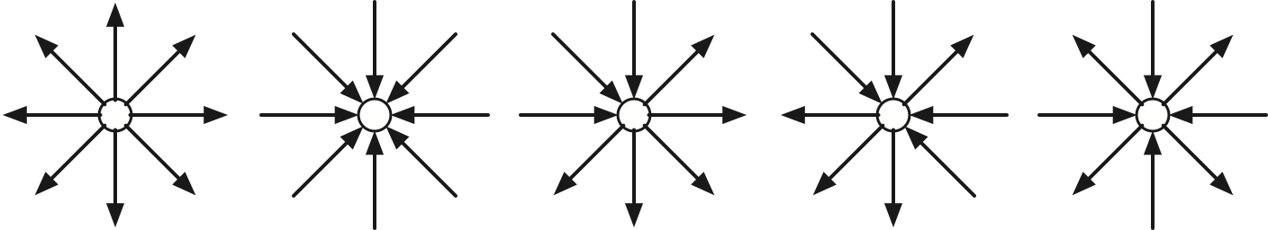
We call a vertex \(v\) in a directed planar map regular if its cycle of incident edges consists of a single interval of incoming edges followed by a single interval of outgoing edges. We call \(v\) a saddle if \(v\) is incident to four edges that are directed into \(v\), out of \(v\), into \(v\), and out of \(v\) in cyclic order around \(v\).1
Prove that a planar graph \(G\) is strongly connected if and only if its dual graph \(G^*\) (with respect to any planar embedding) is acyclic.
Let \(G\) be a directed acyclic planar graph with a unique source \(s\) and a unique sink \(t\). Prove that in every planar embedding of \(G\), every vertex except \(s\) and \(t\) is regular.
Let \(G\) be a (weakly) connected directed acyclic planar graph with \(k\) sources and \(\ell\) sinks. Prove that every planar embedding of \(G\) contains at most \(k+\ell-2\) saddle vertices.
Our proof of the Tutte spring-embedding theorem assumed that every stress coefficient \(\lambda_{u\mathord\to v}\) is positive. But in fact, the theorem extends fairly easily to the setting where some stress coefficients are zero. Zero-weight darts allow us to model directed planar graphs, by identifying directed edges with positive-weight darts. (We still keep the zero-weight darts in our graph data structure for navigational purposes.) A drawing/embedding of a directed graph is a drawing/embedding of its underlying undirected graph; each directed edge corresponds to an orientation of the corresponding undirected edge path.
Find the weakest condition you can for planar graphs with non-negative dart coefficients that implies that the Tutte drawing is a strictly convex embedding. For example, “simple 3-connected planar graph with all positive stress coefficients” is sufficient, but stronger than necessary.
As a starting point, consider planar graphs in which every stress coefficient is either \(0\) or \(1\). Equivalently, consider Tutte drawings of directed planar graphs, where every interior vertex is positioned at the center of mass of its in-neighbors.
The transshipment problem is the uncapacitated special case of the minimum-cost flow problem. A transshipment network consists of a directed graph \(G\), a balance \(b(v)\) for each vertex \(v\), and a cost \(\$(e)\) for each directed edge \(e\). The vertex balances must sum to zero; positive balances are interpreted as demand, and negative balances as supply.
A feasible flow in a transshipment network \((G, b, \$)\) assigns a non-negative real value \(f(e)\) to each directed edge \(e\), such that \(\sum_u f(u\mathord\to v) - \sum_w f(v\mathord\to w) = b(v)\) at every vertex \(v\); that is, the total net flow into \(v\) must equal the balance of \(v\). The goal of the transshipment problem is to compute a feasible flow \(f\) with minimum total cost \(\$(f) = \sum_e \$(e)\cdot f(e)\).
Every transshipment network has a minimum-cost flow that is supported on a spanning tree \(T\), meaning \(f(e)\) for every non-tree edge \(e\). (More generally, every basic feasible solution to the transshipment linear program is a feasible flow supported on a spanning tree.) We can always symbolically perturb the edge costs so that the minimum-cost flow is unique.
The single-source shortest-path problem is the special case of transshipment where the source vertex \(s\) has balance \(1-n\), every other vertex has balance \(1\), and the cost of an edge is its length. The transshipment tree \(T\) is just the shortest path tree rooted at \(s\); if \(u\) is the parent of \(v\) in \(T\), then \(f(u\mathord\to v)\) is equal to the number of descendants of \(v\) (including \(v\) itself).
Now consider the following alternative strategy for the multiple-source shortest path problem. Let \(s_1, s_2, \dots, s_k\) be the vertices on the outer face of the input planar map \(\Sigma\). For each index \(i\), let \(T_i\) denote the transshipment tree for this network when \(b(s_i) = 1-n\) and \(b(v)=1\) for all \(v\ne s_i\). We begin by computing \(T_1\) from scratch (using Dijkstra’s algorithm, for example). Then in the \(i\)th phase, we transform \(T_i\) into \(T_{i+1}\) by linearly interpolating the balances and maintaining a transhipment tree. That is, we maintain the transshipment tree \(T_\lambda\) for the balances \[ b_\lambda(v) = \begin{cases} 1 - n + n\lambda & \text{if $v = s_i$} \\ 1 - n\lambda & \text{if $v = s_{i+1}$} \\ 1 & \text{otherwise} \end{cases} \] as the parameter \(\lambda\) continuously increases from \(0\) to \(1\). Just as in the parametric-shortest-path formulation, the transshipment tree changes at discrete times by pivots: An edge pivots out when its flow value drops to zero, and the minimum-cost edge that reconnects the tree pivots in.
Prove that over the entire algorithm, each directed edge pivots into the transshipment tree at most once and out of the transshipment tree at most once. (Hint: Argue that the sequence of pivots is almost identical to the sequence of parametric shortest-path tree pivots!)
Every vertex in the Nagy graph of a generic plane curve is a saddle.↩︎